Modeling Financial Markets as MDPs

We know that games can be modeled using Markov decision processes and thus be solved using Reinforcement learning algorithms. Can the same reasoning be applied to the financial market? Can financial markets be treated as a game where the utility function is to make more money as possible?

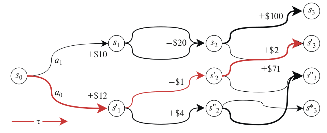
Recent papers told us so. Even though financial markets are not a game, their mechanics can be approximated with a Markov decision process. At each time step \(t \), the agent receives some representation of the environment denoted by S_t. Given this state, an agent chooses an action \( A_t \) and based on this action, a numerical reward \( R_{t+1} \) is given to the agent at the next time step, and the agent finds itself in a new state \( S_t+1 \). The interaction between the agent and the environment produces a trajectory tau. At any time step \( t \), the goal of an RL is to maximize the expected return denoted as \( G_t \) at time \( t \). It is empirically proven that financial assets are extremely dependent on newer events than past events. This is another point on the reasons why financial markets can be modeled with a Markov process: they satisfy the Markov property. The Markov property formally can be defined as:

the conditional probability distribution of future states of the process depends only upon the present state, not on the sequence of events that preceded it. This is always the case with financial markets as they tend to always look forward to what is likely to happen in the future.

The state-space in the case of financial markets is usually represented using the OHLCV data with the addition of various technical indicators of the past n-th days of the target security. The usual technical indicators included are the MACD, the RSI, the ATR, and various moving averages. To make the agent aware of its position on the market and the current PnL, a vector that encodes this kind of information can also be included in the state space. All those data points can be put together in a vectorized fashion and used as the input of the neural net.

Regarding the action space, there are two main ways of implementation: discrete action space: where a simple action set of {-1, 0, 1} (or other types of encoding) is used, to represent sell, hold, and buy action respectively. continuous action space: allow actions to be any value between -1 and 1.

The trickiest part of a reinforcement learning environment to design is the reward function. This could be simply equal to the returns (or log-returns) of the agent trade, which are given only when the agent closes a trade. Or the reward function can be designed to take into account also the risk of each trade. Finding the right reward function might be also based on the goals that want to be obtained by the agent. Giving the plain returns can be a valid option if the goal is to merely optimize the profit, while if the goal is also to obtain a less volatile equity line the reward function must take the risks into account. Consequently, it can be concluded that there is no single way to design a reward function, everyone has to design it according to the set objectives.

To make a concrete example let’s suppose that our environment is the crude oil continuos future. Let’s also suppose that our agent is going to act on daily candles. Apart from the OHLCV data, we want to include two moving averages (a 50-period MA and a 200-period MA), the RSI, the ATR, and a positional encoding of the day and month variables. Since we would like to leverage the implied volatility (implied volatility is one of the only financial data that is forward-looking) on this asset we also would like to include the OHLC data of the OVX index, which is the volatility index of the crude oil futures.

Fixing the input state to the previous 21 trading days at each step we got a input data similar to the following:

             open   high    low  close        MA  Smoothing Line     MA.1  Smoothing Line.1  Volume  Volume MA       ATR        RSI  RSI-based MA  open_ovx  high_ovx  low_ovx  close_ovx       day_sin   day_cos     month_sin  month_cos
Date                                                                                                                                                                                                                                      
2007-05-11  61.89  62.56  61.68  62.37  62.28530        62.40756  62.5848          62.57444  216920  228967.65  1.595914  46.550818     50.353979     26.41     26.41    26.41      26.41  7.431448e-01 -0.669131  5.000000e-01  -0.866025
2007-05-14  62.43  63.07  62.14  62.46  62.23140        62.34749  62.6012          62.58312  200433  227399.15  1.548348  46.999236     49.685978     27.23     27.23    27.23      27.23  2.079117e-01 -0.978148  5.000000e-01  -0.866025
2007-05-15  62.54  63.30  62.07  63.17  62.17525        62.28898  62.6632          62.60072  185334  225779.35  1.525609  50.525568     48.967185     27.89     27.89    27.89      27.89  1.224647e-16 -1.000000  5.000000e-01  -0.866025
2007-05-16  63.15  63.30  61.90  62.55  62.11345        62.23031  62.7004          62.62540  216160  225719.05  1.516637  47.550389     48.298946     27.07     27.07    27.07      27.07 -2.079117e-01 -0.978148  5.000000e-01  -0.866025
2007-05-17  62.62  65.09  62.48  64.86  62.05870        62.17282  62.7612          62.66216  267955  228258.40  1.594734  57.574277     48.023056     24.86     24.86    24.86      24.86 -4.067366e-01 -0.913545  5.000000e-01  -0.866025
2007-05-18  65.90  66.44  65.59  65.98  62.01130        62.11802  62.8480          62.71480  168618  228173.60  1.593682  61.423777     48.273097     24.71     24.71    24.71      24.71 -5.877853e-01 -0.809017  5.000000e-01  -0.866025
2007-05-21  65.94  67.10  65.28  66.87  61.97185        62.06611  62.9844          62.79144  192779  228295.70  1.609848  64.203327     49.123527     24.67     24.67    24.67      24.67 -9.510565e-01 -0.309017  5.000000e-01  -0.866025
2007-05-22  66.80  67.00  65.40  65.51  61.91450        62.01396  63.1164          62.88208  201705  225693.85  1.609144  57.397494     49.690902     26.03     26.03    26.03      26.03 -9.945219e-01 -0.104528  5.000000e-01  -0.866025
2007-05-23  65.61  66.20  65.05  65.77  61.86180        61.96363  63.2732          62.99664  230829  227269.20  1.576348  58.307411     50.458624     26.35     26.35    26.35      26.35 -9.945219e-01  0.104528  5.000000e-01  -0.866025
2007-05-24  65.72  66.15  63.82  64.18  61.80095        61.91208  63.3936          63.12312  212993  227268.00  1.630180  51.117194     51.038639     26.63     26.63    26.63      26.63 -9.510565e-01  0.309017  5.000000e-01  -0.866025
2007-05-25  64.48  65.30  64.21  65.20  61.75695        61.86121  63.5466          63.26284  144492  223578.50  1.593739  54.954752     52.004388     25.81     25.81    25.81      25.81 -8.660254e-01  0.500000  5.000000e-01  -0.866025
2007-05-29  64.98  65.24  62.54  63.15  61.70095        61.80703  63.6180          63.38956  221016  223358.60  1.672758  46.973199     52.136539     27.83     27.83    27.83      27.83 -2.079117e-01  0.978148  5.000000e-01  -0.866025
2007-05-30  63.26  63.87  62.88  63.49  61.65075        61.75428  63.6938          63.50504  215024  220918.55  1.623989  48.314002     52.549657     28.61     28.61    28.61      28.61 -2.449294e-16  1.000000  5.000000e-01  -0.866025
2007-05-31  63.31  64.27  62.43  64.01  61.60555        61.70303  63.7890          63.60820  275955  222738.50  1.639419  50.380481     53.019423     28.44     28.44    28.44      28.44  2.079117e-01  0.978148  5.000000e-01  -0.866025
2007-06-01  64.23  65.25  63.80  65.08  61.57150        61.65714  63.8984          63.70916  225803  223350.60  1.625889  54.418871     53.581427     27.39     27.39    27.39      27.39  2.079117e-01  0.978148  1.224647e-16  -1.000000
2007-06-04  64.87  66.48  64.53  66.21  61.55225        61.61620  63.9888          63.79760  228630  223155.85  1.649039  58.280530     54.387234     27.36     27.36    27.36      27.36  7.431448e-01  0.669131  1.224647e-16  -1.000000
2007-06-05  66.05  66.20  65.23  65.61  61.51980        61.57997  64.0554          63.88508  200804  220771.10  1.601251  55.587605     54.748808     26.70     26.70    26.70      26.70  8.660254e-01  0.500000  1.224647e-16  -1.000000
2007-06-06  65.67  66.31  65.21  65.96  61.48310        61.54644  64.1164          63.96960  222155  217995.55  1.565447  56.840399     55.412380     25.94     25.94    25.94      25.94  9.510565e-01  0.309017  1.224647e-16  -1.000000
2007-06-07  65.90  67.42  65.82  66.93  61.45225        61.51578  64.1964          64.05108  275768  218017.05  1.567915  60.191871     55.599351     26.11     26.11    26.11      26.11  9.945219e-01  0.104528  1.224647e-16  -1.000000
2007-06-08  66.70  66.83  64.56  64.76  61.41725        61.48493  64.2100          64.11340  284370  219387.15  1.625207  50.705761     54.833778     26.51     26.51    26.51      26.51  9.945219e-01 -0.104528  1.224647e-16  -1.000000
2007-06-11  64.70  66.07  64.52  65.97  61.38530        61.45154  64.2088          64.15740  234653  220273.80  1.619835  54.967498     54.174076     25.99     25.99    25.99      25.99  7.431448e-01 -0.669131  1.224647e-16  -1.000000

If we are using a recurrent net this 21x21 input is fine, while if the agent is using a fully connected network this data must be squeezed into a single vector.

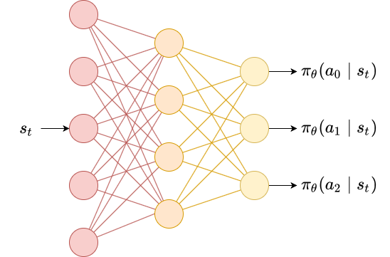
In this environment, only three actions are possible: buy a fixed fraction of the asset (1), sell a fixed fraction of the asset (2), or hold (0). So in case, the policy is parametrized \( \pi_{\theta} \) at each step a probability distribution over its actions is given \( \pi_{\theta}(A | S_t) \). The figure below shows an example.

Assuming that our risk appetite is high, we can design a reward function that is going to maximize the returns no matter what. Let \( cp \) the price of the traded asset at the current step \( i \), and let \( ltp \) the last traded price that is the price we the agent have opened a trade. If the agent position is a long position the current step reward is given by the log-returns that the agent could get by closing the trade:

similarly, if the agent position is a short position the current step reward is

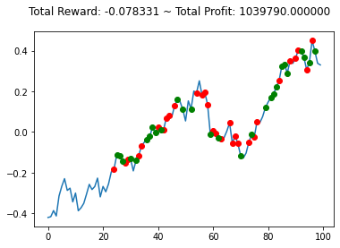
Here’s an example of how our env could work using the openai gym library:

observation = env.reset()
while True:
    action = env.action_space.sample()
    observation, reward, done, info = env.step(action)
    
    if done:
        print("info:", info)
        break

Resulting in:

There are few libraries that implement a Trading environment that can be used for RL algo:

• FinRL: an open-source library for deep reinforcement learning in finance by AI4Finance Foundation. It’s a well-documented library with over 5.6k stars on GitHub.
• gym-anytrading: is a collection of OpenAI Gym environments for reinforcement learning-based trading algorithms. It’s a pretty simple and lightweight library that you could also use to extend the base class and make your own env.
• gym-anytrading-2.0: my fork of gym-anytrading, where I reimplemented the base TradingEnv class in my own way. The main differences from the original projects are in the way the rewards are calculated, position sizing logic has been added, and the Hold action has been added. Further modifications have been planned to make the env even more flexible. Contributors are welcome!

But as pointed out by Tidor-Vlad Pricope in trading, our training, backtesting, and live environments can become so different that we can’t really make any guarantees. Those envs are just for research purpouses and they have to be treated for what they are, and what they can accomplish.

References

• Deep Reinforcement Learning for Trading
• Capturing Financial markets to apply Deep Reinforcement Learning
• Deep Reinforcement Learning in Quantitative Algorithmic Trading: A Review