Paolo's Blog Random thoughts of a Junior Computer Scientist
Building a NG strategy with a Random Forest Regressor
Is it possible to teach an ML model to trade?
The short answer is yes. But how well the model will perform with data it has never seen before?
That’s the big problem with machine learning and also with trading strategies. As we don’t want a trained model to overfit the training data we also don’t want a trading strategy to overfit the in-sample data. The keyword here is robustness. What we are looking for both in trading and machine learning is to build a generalized model. In the case of trading, this means performing well in different assets classes with the same price setup. While In the case of machine learning, this means that our model is not “memorizing” training data, but rather it is “learning” to generalize from a trend.
For more information about the notebook and the data, this is the official github repo.
import warnings

warnings.filterwarnings('ignore')
%matplotlib inline

import numpy as np
import pandas as pd

import matplotlib.pyplot as plt
from matplotlib.ticker import FuncFormatter
from mpl_toolkits.mplot3d import Axes3D
import seaborn as sns

from sklearn.model_selection import BaseCrossValidator
from sklearn.metrics import make_scorer
from sklearn.ensemble import RandomForestRegressor, \
    GradientBoostingRegressor, AdaBoostRegressor
from sklearn.tree import DecisionTreeRegressor
from sklearn.model_selection import cross_val_score

from scipy.stats import spearmanr
dataset_path = '../data/model_data.h5'
Load Data
The dataset is not only composed by OHLCV data, but I’ve also incorporated:
- fundamental data such as the consuption of NG, the storage, …
- technical indicators data such as the RSI, MACD, the ATR, …
- the $n$ lagged returns where $n \in {1, 5, 10, 21, 63}$
- the $n$ forward returns which are the target variables
- variables that are referring to year, month, and weekday
Since I’ve decided to test out Tree based model, I’m going to use this data as I would do for a tipical machine learning task. So the model won’t have a notion of time, just like timeseries model.
data = pd.read_hdf(dataset_path, 'no_dummies')
data = data.drop([c for c in data.columns if 'lag' in c], axis=1)
data
| Close | Volume | Open | High | Low | Consumption in mcf | Storage in mcf | US Gross Withdrawal in mcf | Other Gross Withdrawal in mcf | RSI | ... | return_21d | return_42d | return_63d | target_1d | target_5d | target_10d | target_21d | year | month | weekday | |
|---|---|---|---|---|---|---|---|---|---|---|---|---|---|---|---|---|---|---|---|---|---|
| Date | |||||||||||||||||||||
| 2012-04-09 | 2.107 | 108772.0 | 2.103 | 2.117 | 2.065 | 1953071.0 | 2478.0 | 2417498.0 | 93400.0 | 34.901425 | ... | -0.003584 | -0.003797 | -0.005916 | -0.036070 | -0.015267 | -0.006449 | 0.007501 | 2012 | 4 | 0 |
| 2012-04-10 | 2.031 | 120126.0 | 2.111 | 2.125 | 2.025 | 1953071.0 | 2478.0 | 2417498.0 | 93400.0 | 30.556017 | ... | -0.006397 | -0.004436 | -0.006230 | -0.023634 | -0.008005 | 0.001807 | 0.009692 | 2012 | 4 | 1 |
| 2012-04-12 | 1.983 | 188668.0 | 1.976 | 2.068 | 1.972 | 1953071.0 | 2478.0 | 2417498.0 | 93400.0 | 28.170441 | ... | -0.006395 | -0.005282 | -0.006237 | -0.001009 | -0.007785 | 0.002641 | 0.011266 | 2012 | 4 | 3 |
| 2012-04-13 | 1.981 | 111947.0 | 1.982 | 1.999 | 1.959 | 1953071.0 | 2503.0 | 2417498.0 | 93400.0 | 28.072097 | ... | -0.007064 | -0.005306 | -0.005330 | 0.017668 | -0.005512 | 0.009896 | 0.009795 | 2012 | 4 | 4 |
| 2012-04-16 | 2.016 | 115321.0 | 1.986 | 2.030 | 1.977 | 1953071.0 | 2503.0 | 2417498.0 | 93400.0 | 32.512260 | ... | -0.005926 | -0.004447 | -0.004609 | -0.032242 | -0.000894 | 0.012604 | 0.010299 | 2012 | 4 | 0 |
| ... | ... | ... | ... | ... | ... | ... | ... | ... | ... | ... | ... | ... | ... | ... | ... | ... | ... | ... | ... | ... | ... |
| 2021-08-24 | 3.896 | 54557.0 | 3.929 | 3.970 | 3.884 | 2218011.0 | 2851.0 | 3396062.0 | 32500.0 | 50.393336 | ... | -0.002451 | 0.003121 | 0.004626 | 0.000257 | 0.023556 | 0.023485 | 0.011719 | 2021 | 8 | 1 |
| 2021-08-25 | 3.897 | 37979.0 | 3.900 | 3.991 | 3.858 | 2218011.0 | 2851.0 | 3396062.0 | 32500.0 | 50.456830 | ... | -0.000895 | 0.002589 | 0.004246 | 0.073646 | 0.034399 | 0.025870 | 0.013270 | 2021 | 8 | 2 |
| 2021-08-26 | 4.184 | 64362.0 | 3.917 | 4.217 | 3.896 | 2218011.0 | 2851.0 | 3396062.0 | 32500.0 | 64.500602 | ... | 0.001622 | 0.003632 | 0.005519 | 0.044455 | 0.020949 | 0.016707 | 0.014884 | 2021 | 8 | 3 |
| 2021-08-27 | 4.370 | 3899.0 | 4.202 | 4.397 | 4.197 | 2218011.0 | 2871.0 | 3396062.0 | 32500.0 | 70.363841 | ... | 0.003522 | 0.004427 | 0.006063 | -0.014874 | 0.015184 | 0.018147 | 0.013912 | 2021 | 8 | 4 |
| 2021-08-30 | 4.305 | 161299.0 | 4.499 | 4.526 | 4.222 | 2218011.0 | 2871.0 | 3396062.0 | 32500.0 | 66.246073 | ... | 0.004544 | 0.003937 | 0.005205 | 0.016725 | 0.011930 | 0.020237 | 0.011532 | 2021 | 8 | 0 |
2351 rows × 25 columns
data.info()
<class 'pandas.core.frame.DataFrame'>
DatetimeIndex: 2351 entries, 2012-04-09 to 2021-08-30
Data columns (total 25 columns):
 #   Column                         Non-Null Count  Dtype
---  ------                         --------------  -----
 0   Close                          2351 non-null   float64
 1   Volume                         2351 non-null   float64
 2   Open                           2351 non-null   float64
 3   High                           2351 non-null   float64
 4   Low                            2351 non-null   float64
 5   Consumption in mcf             2351 non-null   float64
 6   Storage in mcf                 2351 non-null   float64
 7   US Gross Withdrawal in mcf     2351 non-null   float64
 8   Other Gross Withdrawal in mcf  2351 non-null   float64
 9   RSI                            2351 non-null   float64
 10  ATR                            2351 non-null   float64
 11  MACD                           2351 non-null   float64
 12  return_1d                      2351 non-null   float64
 13  return_5d                      2351 non-null   float64
 14  return_10d                     2351 non-null   float64
 15  return_21d                     2351 non-null   float64
 16  return_42d                     2351 non-null   float64
 17  return_63d                     2351 non-null   float64
 18  target_1d                      2351 non-null   float64
 19  target_5d                      2351 non-null   float64
 20  target_10d                     2351 non-null   float64
 21  target_21d                     2351 non-null   float64
 22  year                           2351 non-null   int64
 23  month                          2351 non-null   int64
 24  weekday                        2351 non-null   int64
dtypes: float64(22), int64(3)
memory usage: 477.5 KB
def get_X_y(data: pd.DataFrame):
    columns_to_drop = ['Open', 'Close', 'Low', 'High', 'Volume']
    y = data.filter(like='target')
    X = data.drop(columns_to_drop, axis=1)
    X = X.drop(y.columns, axis=1)
    return X, y
X, y = get_X_y(data)
Now that we have out X and y let’s split the data in a trainig set and test set.
The test won’t only be used for testing the final model, but it will be also used for the backtesting part.
X, X_test, y, y_test = X.loc['2012':'2019'], X.loc['2019':'2021'], y.loc['2012':'2019'], y.loc['2019':'2021']
f'Train lenght: {len(X)}', f'Test length: {len(X_test)}'
('Train lenght: 1932', 'Test length: 671')
class MultipleTimeSeriesCV(BaseCrossValidator):
    """Generates tuples of train_idx, test_idx pairs"""

    def __init__(self,
                 n_splits=3,
                 train_period_length=126,
                 test_period_length=21,
                 lookahead=None,
                 shuffle=False):
        self.n_splits = n_splits
        self.lookahead = lookahead
        self.test_length = test_period_length
        self.train_length = train_period_length
        self.shuffle = shuffle

    def split(self, X, y=None, groups=None):
        unique_dates = X.index.get_level_values('Date').unique()
        days = sorted(unique_dates, reverse=True)

        split_idx = []
        for i in range(self.n_splits):
            test_end_idx = i * self.test_length
            test_start_idx = test_end_idx + self.test_length
            train_end_idx = test_start_idx + self.lookahead - 1
            train_start_idx = train_end_idx + self.train_length + self.lookahead - 1
            split_idx.append([train_start_idx, train_end_idx,
                              test_start_idx, test_end_idx])

        dates = X.reset_index()[['Date']]
        for train_start, train_end, test_start, test_end in split_idx:
            train_idx = dates[(dates.Date > days[train_start])
                              & (dates.Date <= days[train_end])].index
            test_idx = dates[(dates.Date > days[test_start])
                             & (dates.Date <= days[test_end])].index
            if self.shuffle:
                np.random.shuffle(list(train_idx))
            yield train_idx, test_idx

    def get_n_splits(self, X=None, y=None, groups=None):
        return self.n_splits
n_splits = 15
train_period_length = 300
test_period_length = 100
lookaheads = [1, 5, 10, 21]
# Utilities functions

def display_score(scores):
    print('scores: ',scores)
    print('mean: ', scores.mean())
    print('standard deviation: ', scores.std())


def rank_correl(y, y_pred):
    return spearmanr(y, y_pred, axis=None)[0]

ic = make_scorer(rank_correl)


def get_cross_val_score(model, X, y, score_fun, cv, n_jobs=-1):
    cv_score = cross_val_score(estimator=model,
                           X=X,
                           y=y,
                           scoring=score_fun,
                           cv=cv,
                           n_jobs=n_jobs,
                           verbose=1)
    display_score(cv_score)
The scoring function that we are going to use to test out the models is the spearman correlation $\rho$. But why are we using this kind of correlation in first place?
Unlike the tipical loss function that are used in machine learning, the spearman correlation assesses how well the relationship between two variables can be described usign a monotonic function.
If the pearson correlation gives a perfect value when $X$ and $Y$ are related by a linear function, the spearman correlation results when $X$ and $Y$ are related by any monotonic function.
Here’s and example:
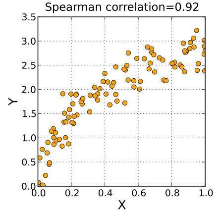
Form the image above we can see that the spearman correlation is high even though there isn’t a linear correlation between $X$ and $Y$. In fact we can intuitevily see that $Y = \sqrt{c X}$
Let’s now test out which is the best tree model using the spearman correlation as a scoring function.
Decision Tree Regressor
dt_reg = DecisionTreeRegressor(max_depth=None,
                               min_samples_split=2,
                               min_samples_leaf=1,
                               max_features='auto')
for lookahead in lookaheads:
    cv = MultipleTimeSeriesCV(n_splits=n_splits,
                          train_period_length=train_period_length,
                          test_period_length=test_period_length,
                          lookahead=lookahead)
    print(f'lookhead: {lookahead}')
    get_cross_val_score(dt_reg, X, y, ic, cv)
    print('\n')
lookhead: 1


[Parallel(n_jobs=-1)]: Using backend LokyBackend with 3 concurrent workers.
[Parallel(n_jobs=-1)]: Done  15 out of  15 | elapsed:    2.6s finished
[Parallel(n_jobs=-1)]: Using backend LokyBackend with 3 concurrent workers.


scores:  [-0.13101391  0.15451854  0.18070339 -0.0562517  -0.03433135  0.06979087
  0.09453872  0.11061872 -0.04106021  0.11633454  0.18392795  0.14913466
  0.02506414  0.0346177   0.16230884]
mean:  0.06792672580348139
standard deviation:  0.09463351327402522


lookhead: 5


[Parallel(n_jobs=-1)]: Done  10 out of  15 | elapsed:    0.3s remaining:    0.1s
[Parallel(n_jobs=-1)]: Done  15 out of  15 | elapsed:    0.3s finished
[Parallel(n_jobs=-1)]: Using backend LokyBackend with 3 concurrent workers.
[Parallel(n_jobs=-1)]: Done  10 out of  15 | elapsed:    0.1s remaining:    0.1s
[Parallel(n_jobs=-1)]: Done  15 out of  15 | elapsed:    0.2s finished
[Parallel(n_jobs=-1)]: Using backend LokyBackend with 3 concurrent workers.


scores:  [-0.20927668  0.04604246  0.09179215 -0.08948434  0.05706104  0.12117565
  0.09213837  0.05793836 -0.01934843  0.11038874 -0.01854846 -0.08714146
  0.14893241  0.04732402 -0.06412406]
mean:  0.018991318379871048
standard deviation:  0.0951334842919218


lookhead: 10
scores:  [-0.19912898  0.12238416  0.04419881 -0.1036148   0.07946813  0.02062854
  0.06730263  0.30685917  0.0606858   0.1000542  -0.06519469 -0.04041847
  0.05410469  0.08347365  0.00963497]
mean:  0.03602918631257569
standard deviation:  0.11040736275079402


lookhead: 21
scores:  [-0.10136783  0.08902033  0.1383936   0.09122781  0.03461467 -0.06061215
 -0.02665178  0.0537336   0.08048373 -0.03661694  0.04605128  0.01691698
  0.02963777 -0.06728841 -0.03722724]
mean:  0.01668769340217639
standard deviation:  0.06682570728253841


[Parallel(n_jobs=-1)]: Done  10 out of  15 | elapsed:    0.1s remaining:    0.1s
[Parallel(n_jobs=-1)]: Done  15 out of  15 | elapsed:    0.1s finished
Random Forest Regressor
rf_reg = RandomForestRegressor(n_estimators=100,
                                max_depth=None,
                                min_samples_split=2,
                                min_samples_leaf=1,
                                min_weight_fraction_leaf=0.0,
                                max_features='auto',
                                max_leaf_nodes=None,
                                min_impurity_decrease=0.0,
                                bootstrap=True,
                                oob_score=False,
                                n_jobs=-1,
                                random_state=None,
                                verbose=0,
                                warm_start=False)
for lookahead in lookaheads:
    cv = MultipleTimeSeriesCV(n_splits=n_splits,
                          train_period_length=train_period_length,
                          test_period_length=test_period_length,
                          lookahead=lookahead)
    print(f'lookhead: {lookahead}')
    get_cross_val_score(rf_reg, X, y, ic, cv)
    print('\n')
[Parallel(n_jobs=-1)]: Using backend LokyBackend with 3 concurrent workers.


lookhead: 1


[Parallel(n_jobs=-1)]: Done  15 out of  15 | elapsed:    4.4s finished
[Parallel(n_jobs=-1)]: Using backend LokyBackend with 3 concurrent workers.


scores:  [-0.13863668  0.30713462  0.28466835 -0.09170711  0.11769505  0.15852962
  0.08962024  0.15531941  0.04524835  0.15721646 -0.00053663  0.14467668
  0.07360171  0.12293946  0.18112238]
mean:  0.10712612712307454
standard deviation:  0.1163415452886651


lookhead: 5


[Parallel(n_jobs=-1)]: Done  15 out of  15 | elapsed:    3.1s finished
[Parallel(n_jobs=-1)]: Using backend LokyBackend with 3 concurrent workers.


scores:  [-1.60942756e-01  2.85937238e-01  2.85947202e-01 -3.43541538e-02
  9.48986556e-02  1.59270620e-01  1.02904417e-01  1.50913881e-01
  1.65938568e-04  1.28500090e-01  1.22980144e-02  1.83860871e-01
  8.17587610e-02  1.23204020e-01  1.59399434e-01]
mean:  0.10491748226609333
standard deviation:  0.11283350114033273


lookhead: 10


[Parallel(n_jobs=-1)]: Done  15 out of  15 | elapsed:    4.6s finished
[Parallel(n_jobs=-1)]: Using backend LokyBackend with 3 concurrent workers.


scores:  [-0.15371946  0.31925742  0.2579257  -0.0432299   0.08924062  0.09395159
  0.18299472  0.15148163  0.05348772  0.09191036  0.04119813  0.12714026
  0.10451165  0.10017288  0.04291752]
mean:  0.09728272234414333
standard deviation:  0.10868445700120122


lookhead: 21
scores:  [-0.07855662  0.2605627   0.17725544  0.10996082  0.10711267  0.02077194
  0.08216481  0.11132113  0.07765269  0.04165095  0.02646954  0.08661731
  0.09749236  0.1256451   0.09840193]
mean:  0.08963485163230227
standard deviation:  0.07259440406955318


[Parallel(n_jobs=-1)]: Done  15 out of  15 | elapsed:    3.6s finished
Gradient Boosting Regressor
grad_reg = GradientBoostingRegressor(n_estimators=250,
                                        max_depth=None,
                                        min_samples_split=2,
                                        min_samples_leaf=1,
                                        min_weight_fraction_leaf=0.0,
                                        max_features='auto',
                                        max_leaf_nodes=None,
                                        min_impurity_decrease=0.0,
                                        random_state=None,
                                        verbose=0,
                                        warm_start=False)
for lookahead in lookaheads:
    cv = MultipleTimeSeriesCV(n_splits=n_splits,
                          train_period_length=train_period_length,
                          test_period_length=test_period_length,
                          lookahead=lookahead)
    print(f'lookhead: {lookahead}')
    get_cross_val_score(grad_reg, X, y[f'target_{lookahead}d'], ic, cv)
    print('\n')
[Parallel(n_jobs=-1)]: Using backend LokyBackend with 3 concurrent workers.


lookhead: 1


[Parallel(n_jobs=-1)]: Done  15 out of  15 | elapsed:    5.9s finished
[Parallel(n_jobs=-1)]: Using backend LokyBackend with 3 concurrent workers.


scores:  [-0.20445306  0.01328533  0.16203015 -0.00838286  0.02444644  0.19617162
 -0.00039004  0.01285329  0.02569495  0.28550855  0.01215722 -0.05161132
  0.10326464  0.18349835 -0.02442244]
mean:  0.048643387344077575
standard deviation:  0.1160384340548671


lookhead: 5


[Parallel(n_jobs=-1)]: Done  15 out of  15 | elapsed:    4.8s finished
[Parallel(n_jobs=-1)]: Using backend LokyBackend with 3 concurrent workers.


scores:  [-0.39282189  0.05045305 -0.02626936 -0.20777678 -0.01662166  0.11324502
 -0.06610281  0.21798576 -0.05822539  0.09680168  0.17827997 -0.06715872
  0.14292229  0.00322832 -0.04282028]
mean:  -0.004992052919846818
standard deviation:  0.14981225481196084


lookhead: 10


[Parallel(n_jobs=-1)]: Done  15 out of  15 | elapsed:    4.6s finished
[Parallel(n_jobs=-1)]: Using backend LokyBackend with 3 concurrent workers.


scores:  [-0.30514475  0.26224452  0.04842499  0.00207621  0.15526646  0.2469607
  0.12970897 -0.04288132  0.49446886 -0.00571257  0.24380204 -0.15146387
  0.09441372  0.20837809 -0.22545455]
mean:  0.07700583284484216
standard deviation:  0.20151505597435154


lookhead: 21
scores:  [-0.16522151 -0.39272963  0.2310718   0.19308731  0.27021902  0.43274657
 -0.4213874  -0.55196416  0.23484019 -0.04939124 -0.10160734 -0.11212755
 -0.02024669  0.20687669  0.46304047]
mean:  0.014480434762936234
standard deviation:  0.29996516102650683


[Parallel(n_jobs=-1)]: Done  15 out of  15 | elapsed:    2.8s finished
It seems like that the most robust learner is the RandomTreesRegressor, since there is not much deviation using the
various targets. Let’s fine tune it in order to find the bests parameters
Hyperparamter Options
n_estimators = [100, 250]
max_depth = [5, 15, None]
min_samples_leaf = [5, 25, 100]
from itertools import product

cv_params = list(product(n_estimators,
                         max_depth,
                         min_samples_leaf))
n_cv_params = len(cv_params)
n_cv_params
18
sample_proportion = .6
sample_size = int(sample_proportion * n_cv_params)

cv_param_sample = np.random.choice(list(range(n_cv_params)),
                                     size=int(sample_size),
                                     replace=False)
cv_params_ = [cv_params[i] for i in cv_param_sample]
print('# CV parameters:', len(cv_params_))
# CV parameters: 10
Train/Test Period Lenghts
YEAR = 252
train_lengths = [5 * YEAR, 3 * YEAR, YEAR, 126, 63]
test_lengths = [5, 21]
test_params = list(product(train_lengths, test_lengths))
n_test_params = len(test_params)
print('# period params: ', n_test_params)
# period params: 10
Run cross-validation
labels = sorted(y.columns)
features = X.columns.tolist()
lookaheads = [1, 5, 10, 21]
label_dict = dict(zip(lookaheads, labels))
cross_val_cols = [
    'train_length',
    'test_length',
    'n_estimators',
    'max_depth',
    'min_samples_leaf',
    'mean_ic',
    'std_ic',
    'rounds',
    'target'
]

cross_val_results = pd.DataFrame(columns=cross_val_cols)
run_cross_val = False

if run_cross_val:
    for lookahead in lookaheads:
        for train_length, test_length in test_params:
            n_splits = int(7 * YEAR / (train_length + test_length))
            res_row = dict(zip(cross_val_results, [None] * len(cross_val_results)))

            cv = MultipleTimeSeriesCV(n_splits=n_splits,
                                      test_period_length=test_length,
                                      train_period_length=train_length,
                                      lookahead=lookahead)

            res_row['target'] = lookahead
            res_row['train_length'] = train_length
            res_row['test_length'] = test_length


            for p, (n_estimator, max_d, min_s_l) in enumerate(cv_params_):
                base_params = rf_reg.get_params()
                model = RandomForestRegressor(base_params)
                model_params = {
                    'n_estimators': n_estimator,
                    'max_depth': max_d,
                    'max_features': 'log2',
                    'min_samples_leaf': min_s_l
                }
                model = model.set_params(**model_params)

                cval_score = cross_val_score(
                    estimator=model,
                    X=X,
                    y=y,
                    cv=cv,
                    n_jobs=-1,
                    scoring=ic
                )

                for k, v in model_params.items():
                    res_row[k] = v

                res_row['mean_ic'] = cval_score.mean()
                res_row['std_ic'] = cval_score.std()
                res_row['rounds'] = len(cval_score)
                cross_val_results = cross_val_results.append(res_row, ignore_index=True)
                print(f'Lookback: {lookahead}, Train size: {train_length}, Test size: {test_length} ' + \
                      f'# estimators: {n_estimator}, max depth: {max_d}, min samples leaf: {min_s_l}, ic: {cval_score.mean()}')
save = False

if save:
    cross_val_results.to_hdf('./rf_cross_val_results.h5', 'res', mode='w')
load = True

if load:
    cross_val_results = pd.read_hdf('./rf_cross_val_results.h5', 'res')
    cross_val_results.drop('max_features', axis=1, inplace=True)
cross_val_results.head()
| mean_ic | std_ic | ||||||||||||||||
|---|---|---|---|---|---|---|---|---|---|---|---|---|---|---|---|---|---|
| count | mean | std | min | 25% | 50% | 75% | max | count | mean | std | min | 25% | 50% | 75% | max | ||
| train_length | test_length | ||||||||||||||||
| 63 | 5 | 40.0 | -0.040000 | 0.081078 | -0.137663 | -0.097139 | -0.082502 | 0.038680 | 0.106099 | 40.0 | 0.312388 | 0.013639 | 0.284262 | 0.300236 | 0.311043 | 0.325020 | 0.345137 |
| 21 | 40.0 | 0.019963 | 0.047568 | -0.049312 | -0.028885 | 0.025526 | 0.063457 | 0.091317 | 40.0 | 0.137543 | 0.030329 | 0.092126 | 0.109741 | 0.132114 | 0.158911 | 0.204503 | |
| 126 | 5 | 40.0 | -0.001472 | 0.062014 | -0.138518 | -0.040070 | -0.000937 | 0.053062 | 0.099942 | 40.0 | 0.317845 | 0.014023 | 0.286717 | 0.309783 | 0.317301 | 0.326947 | 0.344797 |
| 21 | 40.0 | 0.052328 | 0.042210 | -0.040017 | 0.007511 | 0.067954 | 0.082744 | 0.101916 | 40.0 | 0.158644 | 0.034644 | 0.101250 | 0.124148 | 0.153635 | 0.185232 | 0.225217 | |
| 252 | 5 | 40.0 | 0.013732 | 0.083639 | -0.174116 | -0.013137 | 0.031104 | 0.071588 | 0.134798 | 40.0 | 0.311959 | 0.016541 | 0.268482 | 0.301258 | 0.313738 | 0.319613 | 0.352641 |
| 21 | 40.0 | 0.059629 | 0.064671 | -0.076905 | -0.007141 | 0.083836 | 0.105530 | 0.153957 | 40.0 | 0.168644 | 0.042207 | 0.090941 | 0.116665 | 0.187859 | 0.200833 | 0.218862 | |
| 756 | 5 | 40.0 | 0.093385 | 0.039002 | 0.006339 | 0.060498 | 0.098753 | 0.126201 | 0.152640 | 40.0 | 0.315169 | 0.020823 | 0.274168 | 0.299033 | 0.318346 | 0.328555 | 0.364217 |
| 21 | 40.0 | 0.119656 | 0.025969 | 0.079235 | 0.099342 | 0.115937 | 0.140064 | 0.161495 | 40.0 | 0.188850 | 0.009080 | 0.168275 | 0.184229 | 0.190082 | 0.194146 | 0.210536 | |
| 1260 | 5 | 40.0 | 0.093835 | 0.043284 | 0.001723 | 0.064281 | 0.107727 | 0.127938 | 0.167663 | 40.0 | 0.324773 | 0.018168 | 0.287751 | 0.312535 | 0.325990 | 0.338086 | 0.363679 |
| 21 | 40.0 | 0.143335 | 0.029459 | 0.093199 | 0.118507 | 0.146548 | 0.163117 | 0.193948 | 40.0 | 0.206358 | 0.015252 | 0.173556 | 0.197984 | 0.207888 | 0.216628 | 0.233334 | |
Hyperparameters Analysis
Now that we have our cross validation results, let’s see which hyperparameters combination gives us the best results in various target periods.
First thing first, we would like to understand which train and test period lengths gives the best results. We can do it
by grouping by the train_length and test_length.
tt_lenght_res = cross_val_results.groupby(by=['train_length', 'test_length'])

tt_lenght_res.describe()
| mean_ic | std_ic | ||||||||||||||||
|---|---|---|---|---|---|---|---|---|---|---|---|---|---|---|---|---|---|
| count | mean | std | min | 25% | 50% | 75% | max | count | mean | std | min | 25% | 50% | 75% | max | ||
| train_length | test_length | ||||||||||||||||
| 63 | 5 | 40.0 | -0.067284 | 0.125394 | -0.238227 | -0.198366 | -0.060339 | 0.040526 | 0.175820 | 40.0 | 0.323679 | 0.038303 | 0.247583 | 0.291036 | 0.332345 | 0.355690 | 0.389807 |
| 21 | 40.0 | 0.013003 | 0.045987 | -0.059556 | -0.031805 | 0.020466 | 0.051996 | 0.087472 | 40.0 | 0.141557 | 0.029460 | 0.102602 | 0.110236 | 0.143732 | 0.159184 | 0.204857 | |
| 126 | 5 | 40.0 | 0.037978 | 0.095936 | -0.179574 | -0.037138 | 0.068006 | 0.099740 | 0.182765 | 40.0 | 0.308713 | 0.047910 | 0.210200 | 0.281005 | 0.313996 | 0.345437 | 0.395579 |
| 21 | 40.0 | 0.034013 | 0.031098 | -0.029292 | 0.013257 | 0.033019 | 0.056213 | 0.100750 | 40.0 | 0.142778 | 0.035196 | 0.089118 | 0.103313 | 0.151955 | 0.172974 | 0.196788 | |
| 252 | 5 | 40.0 | 0.099102 | 0.146178 | -0.118797 | -0.035965 | 0.088972 | 0.240602 | 0.344110 | 40.0 | 0.226119 | 0.085731 | 0.057937 | 0.154616 | 0.235666 | 0.275010 | 0.403241 |
| 21 | 40.0 | -0.004490 | 0.070845 | -0.100003 | -0.059219 | -0.007356 | 0.033678 | 0.198329 | 40.0 | 0.175353 | 0.064942 | 0.074036 | 0.093632 | 0.202344 | 0.219997 | 0.280459 | |
| 756 | 5 | 40.0 | 0.186015 | 0.115528 | -0.008271 | 0.110150 | 0.192105 | 0.265226 | 0.460150 | 40.0 | 0.184398 | 0.117764 | 0.005263 | 0.063910 | 0.192105 | 0.283083 | 0.420301 |
| 21 | 40.0 | 0.201002 | 0.105924 | 0.005477 | 0.111770 | 0.197202 | 0.285152 | 0.395819 | 40.0 | 0.053943 | 0.033933 | 0.003493 | 0.023585 | 0.055524 | 0.073221 | 0.146188 | |
| 1260 | 5 | 40.0 | 0.433759 | 0.144668 | -0.111278 | 0.372932 | 0.475188 | 0.501128 | 0.658647 | 40.0 | 0.000000 | 0.000000 | 0.000000 | 0.000000 | 0.000000 | 0.000000 | 0.000000 |
| 21 | 40.0 | 0.362641 | 0.080246 | 0.172502 | 0.317272 | 0.368462 | 0.428501 | 0.512524 | 40.0 | 0.000000 | 0.000000 | 0.000000 | 0.000000 | 0.000000 | 0.000000 | 0.000000 | |
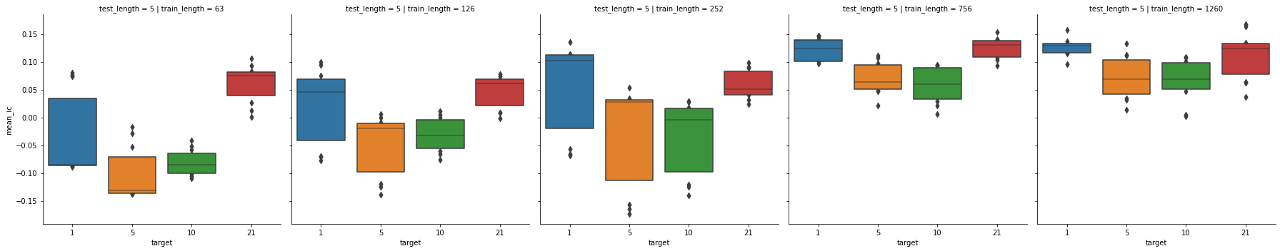
sns.catplot(x='target',
            y='mean_ic',
            col='train_length',
            row='test_length',
            data=cross_val_results[(cross_val_results.test_length == 5)],
            kind='boxen')
<seaborn.axisgrid.FacetGrid at 0x7f74f9aa0490>
sns.catplot(x='target',
            y='mean_ic',
            col='train_length',
            row='test_length',
            data=cross_val_results[(cross_val_results.test_length == 21)],
            kind='boxen')
<seaborn.axisgrid.FacetGrid at 0x7f74f90135e0>

As we can see the longer the train periods are the better, the mean_ic steadly grows as the train period grows. If
we look also to the test period the previous logic is still valid.
Regarding the standard deviation of the ic we can see a great decrease when the test length is longer, while the
train period doesn’t seem to affect positively the standard deviation.
hyperparam_res = cross_val_results.groupby(by=['n_estimators', 'max_depth', 'min_samples_leaf'])

hyperparam_res.describe()
| mean_ic | std_ic | |||||||||||||||||
|---|---|---|---|---|---|---|---|---|---|---|---|---|---|---|---|---|---|---|
| count | mean | std | min | 25% | 50% | 75% | max | count | mean | std | min | 25% | 50% | 75% | max | |||
| n_estimators | max_depth | min_samples_leaf | ||||||||||||||||
| 100 | 5 | 5 | 40.0 | 0.066938 | 0.052099 | -0.058190 | 0.039183 | 0.075439 | 0.101053 | 0.156346 | 40.0 | 0.246668 | 0.067964 | 0.143428 | 0.188625 | 0.246664 | 0.313597 | 0.333802 |
| 25 | 40.0 | 0.073853 | 0.072692 | -0.133699 | 0.041800 | 0.088125 | 0.129480 | 0.179748 | 40.0 | 0.252279 | 0.076549 | 0.099890 | 0.188669 | 0.259033 | 0.323373 | 0.352929 | ||
| 100 | 40.0 | 0.018686 | 0.094137 | -0.174116 | -0.047659 | 0.011730 | 0.101930 | 0.190211 | 40.0 | 0.227733 | 0.090415 | 0.090941 | 0.121915 | 0.246673 | 0.311159 | 0.338839 | ||
| 15 | 5 | 40.0 | 0.067137 | 0.049123 | -0.052001 | 0.045625 | 0.076540 | 0.103037 | 0.153957 | 40.0 | 0.245776 | 0.066883 | 0.139524 | 0.185994 | 0.255743 | 0.306251 | 0.352641 | |
| 25 | 40.0 | 0.069342 | 0.070042 | -0.125135 | 0.033184 | 0.083357 | 0.122653 | 0.156643 | 40.0 | 0.252782 | 0.077793 | 0.110143 | 0.189705 | 0.261310 | 0.325075 | 0.364217 | ||
| 250 | 5 | 100 | 40.0 | 0.023609 | 0.098867 | -0.157054 | -0.051136 | 0.010491 | 0.102668 | 0.193948 | 40.0 | 0.229805 | 0.087395 | 0.101609 | 0.123763 | 0.257245 | 0.310763 | 0.337009 |
| 15 | 5 | 40.0 | 0.070288 | 0.046894 | -0.042150 | 0.047507 | 0.084765 | 0.099238 | 0.145002 | 40.0 | 0.251626 | 0.066471 | 0.145401 | 0.194981 | 0.253222 | 0.317341 | 0.346149 | |
| 25 | 40.0 | 0.071032 | 0.072196 | -0.137299 | 0.041237 | 0.079695 | 0.127785 | 0.158759 | 40.0 | 0.251367 | 0.075597 | 0.100953 | 0.188811 | 0.260109 | 0.326533 | 0.337836 | ||
| 100 | 40.0 | 0.020583 | 0.097593 | -0.164422 | -0.048372 | 0.005453 | 0.101662 | 0.183224 | 40.0 | 0.229869 | 0.090323 | 0.092126 | 0.124280 | 0.250908 | 0.313082 | 0.345137 | ||
By giving a first look to the hyperparameters results, we can see that a larger number of estimators
often gives better ic, while is not really clear what kind of impact the others two parameters have.
It seems like that a lower number of sample for each leaf often gives a greater ic. Let’s see if that it is true by
seeing which combination of parameters gives the highest mean ic.
hyperparam_res.apply(lambda x : x.nlargest(3, 'mean_ic')).drop(['n_estimators', 'max_depth', 'min_samples_leaf'], axis=1)
| train_length | test_length | mean_ic | std_ic | rounds | target | ||||
|---|---|---|---|---|---|---|---|---|---|
| n_estimators | max_depth | min_samples_leaf | |||||||
| 100 | 5 | 5 | 317 | 1260 | 21 | 0.156346 | 0.186483 | 24 | 21 |
| 327 | 756 | 5 | 0.139911 | 0.322106 | 100 | 21 | |||
| 17 | 1260 | 21 | 0.132851 | 0.181271 | 24 | 1 | |||
| 25 | 319 | 1260 | 21 | 0.179748 | 0.187960 | 24 | 21 | ||
| 339 | 756 | 21 | 0.161495 | 0.188905 | 24 | 21 | |||
| 39 | 756 | 21 | 0.158831 | 0.194077 | 24 | 1 | |||
| 100 | 310 | 1260 | 21 | 0.190211 | 0.215878 | 24 | 21 | ||
| 210 | 1260 | 21 | 0.160654 | 0.210699 | 24 | 10 | |||
| 10 | 1260 | 21 | 0.159081 | 0.182454 | 24 | 1 | |||
| 15 | 5 | 55 | 252 | 21 | 0.153957 | 0.178335 | 24 | 1 | |
| 35 | 756 | 21 | 0.127312 | 0.176854 | 24 | 1 | |||
| 25 | 756 | 5 | 0.122724 | 0.281899 | 100 | 1 | |||
| 25 | 334 | 756 | 21 | 0.156643 | 0.191982 | 24 | 21 | ||
| 34 | 756 | 21 | 0.156446 | 0.196219 | 24 | 1 | |||
| 14 | 1260 | 21 | 0.145568 | 0.173556 | 24 | 1 | |||
| 250 | 5 | 100 | 116 | 1260 | 21 | 0.193948 | 0.221515 | 24 | 5 |
| 16 | 1260 | 21 | 0.186957 | 0.214005 | 24 | 1 | |||
| 316 | 1260 | 21 | 0.186653 | 0.224417 | 24 | 21 | |||
| 15 | 5 | 23 | 756 | 5 | 0.145002 | 0.274168 | 100 | 1 | |
| 53 | 252 | 21 | 0.139733 | 0.194309 | 24 | 1 | |||
| 43 | 252 | 5 | 0.134798 | 0.290483 | 100 | 1 | |||
| 25 | 312 | 1260 | 21 | 0.158759 | 0.217793 | 24 | 21 | ||
| 32 | 756 | 21 | 0.157359 | 0.171184 | 24 | 1 | |||
| 322 | 756 | 5 | 0.152640 | 0.331508 | 100 | 21 | |||
| 100 | 11 | 1260 | 21 | 0.183224 | 0.208548 | 24 | 1 | ||
| 311 | 1260 | 21 | 0.176749 | 0.233334 | 24 | 21 | |||
| 111 | 1260 | 21 | 0.172912 | 0.223386 | 24 | 5 |
From the table above we can see that the combinations which gives the best results are {'n_estimators': 100, 'max_depth':5, 'min_samples_leaf': 100} and
{'n_estimators': 250, 'max_depth':5, 'min_samples_leaf': 100}.
n_estimators parameter doesn’t seem to make a big difference in the model, since the result that
we get from the combinations cited above are almost the same, indeed the model with fewer trees performs better
than the one with more trees.
res_target = cross_val_results.groupby(by='target')

res_target.describe()
| mean_ic | std_ic | |||||||||||||||
|---|---|---|---|---|---|---|---|---|---|---|---|---|---|---|---|---|
| count | mean | std | min | 25% | 50% | 75% | max | count | mean | std | min | 25% | 50% | 75% | max | |
| target | ||||||||||||||||
| 1 | 100.0 | 0.066426 | 0.082785 | -0.088416 | -0.030319 | 0.098984 | 0.127388 | 0.186957 | 100.0 | 0.232965 | 0.076905 | 0.099890 | 0.174340 | 0.245204 | 0.301679 | 0.341082 |
| 5 | 100.0 | 0.031137 | 0.085663 | -0.174116 | -0.021445 | 0.054681 | 0.093263 | 0.193948 | 100.0 | 0.243519 | 0.074021 | 0.106925 | 0.188271 | 0.245934 | 0.310896 | 0.363679 |
| 10 | 100.0 | 0.037146 | 0.073816 | -0.139836 | -0.003876 | 0.048050 | 0.092977 | 0.169536 | 100.0 | 0.252171 | 0.077760 | 0.108536 | 0.190572 | 0.263291 | 0.325020 | 0.359887 |
| 21 | 100.0 | 0.087047 | 0.050165 | -0.012699 | 0.057481 | 0.091125 | 0.119924 | 0.190211 | 100.0 | 0.248214 | 0.082655 | 0.090941 | 0.184616 | 0.264477 | 0.323795 | 0.364217 |
ax = sns.boxenplot(x='target', y='mean_ic', data=cross_val_results)
ax.axhline(0, ls='--', lw=1, c='k')
<matplotlib.lines.Line2D at 0x7f74f8d720d0>
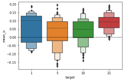
Now that we’ve grouped by target (the lookhead of our model) let’s see that our previous hypothesis about the best hyperparameters that we’ve done before are confirmed.
res_target.apply(lambda x: x.nlargest(3, 'mean_ic')).drop('target', axis=1)
| train_length | test_length | n_estimators | max_depth | min_samples_leaf | mean_ic | std_ic | rounds | ||
|---|---|---|---|---|---|---|---|---|---|
| target | |||||||||
| 1 | 16 | 1260 | 21 | 250 | 5 | 100 | 0.186957 | 0.214005 | 24 |
| 11 | 1260 | 21 | 250 | 15 | 100 | 0.183224 | 0.208548 | 24 | |
| 10 | 1260 | 21 | 100 | 5 | 100 | 0.159081 | 0.182454 | 24 | |
| 5 | 116 | 1260 | 21 | 250 | 5 | 100 | 0.193948 | 0.221515 | 24 |
| 111 | 1260 | 21 | 250 | 15 | 100 | 0.172912 | 0.223386 | 24 | |
| 110 | 1260 | 21 | 100 | 5 | 100 | 0.149622 | 0.213381 | 24 | |
| 10 | 211 | 1260 | 21 | 250 | 15 | 100 | 0.169536 | 0.224359 | 24 |
| 216 | 1260 | 21 | 250 | 5 | 100 | 0.167021 | 0.218431 | 24 | |
| 210 | 1260 | 21 | 100 | 5 | 100 | 0.160654 | 0.210699 | 24 | |
| 21 | 310 | 1260 | 21 | 100 | 5 | 100 | 0.190211 | 0.215878 | 24 |
| 316 | 1260 | 21 | 250 | 5 | 100 | 0.186653 | 0.224417 | 24 | |
| 319 | 1260 | 21 | 100 | 5 | 25 | 0.179748 | 0.187960 | 24 |
res_std = cross_val_results[cross_val_results.std_ic != 0.0].groupby(by='target')
res_std.apply(lambda x: x.nsmallest(3, 'std_ic')).drop('target', axis=1)
| train_length | test_length | n_estimators | max_depth | min_samples_leaf | mean_ic | std_ic | rounds | ||
|---|---|---|---|---|---|---|---|---|---|
| target | |||||||||
| 1 | 99 | 63 | 21 | 100 | 5 | 25 | -0.040090 | 0.099890 | 24 |
| 98 | 63 | 21 | 250 | None | 25 | -0.049312 | 0.100781 | 24 | |
| 92 | 63 | 21 | 250 | 15 | 25 | -0.048031 | 0.100953 | 24 | |
| 5 | 151 | 252 | 21 | 250 | 15 | 100 | -0.032405 | 0.106925 | 24 |
| 150 | 252 | 21 | 100 | 5 | 100 | -0.021299 | 0.115925 | 24 | |
| 156 | 252 | 21 | 250 | 5 | 100 | -0.029880 | 0.118468 | 24 | |
| 10 | 296 | 63 | 21 | 250 | 5 | 100 | 0.012607 | 0.108536 | 24 |
| 250 | 252 | 21 | 100 | 5 | 100 | -0.009350 | 0.112099 | 24 | |
| 271 | 126 | 21 | 250 | 15 | 100 | 0.004410 | 0.114365 | 24 | |
| 21 | 350 | 252 | 21 | 100 | 5 | 100 | -0.012699 | 0.090941 | 24 |
| 391 | 63 | 21 | 250 | 15 | 100 | 0.015370 | 0.092126 | 24 | |
| 351 | 252 | 21 | 250 | 15 | 100 | -0.006404 | 0.095580 | 24 |
From the table above we can see that one of the two best models that we’ve identified before appears three out of the four times in the ranking of the first 3 models.
The hyperparameters of the best model are:
{'n_estimators': 250, 'max_depth':5, 'min_samples_leaf': 100, train_length: 1260, test_length:21}
base_params = rf_reg.get_params()
model = RandomForestRegressor(base_params)
model_params = {
    'n_estimators': 250,
    'max_depth': 5,
    'max_features': 'log2',
    'min_samples_leaf': 100
}
model = model.set_params(**model_params)
opt_test_length = 21
opt_train_length = 1260
scores = np.array([])

for lookahead in lookaheads:
    n_splits = int(2 * YEAR /  opt_test_length)
    cv = MultipleTimeSeriesCV(
        n_splits=n_splits,
        test_period_length=opt_test_length,
        train_period_length=opt_train_length,
        lookahead=lookahead
    )

    for i, (train_idx, test_idx) in enumerate(cv.split(X)):
        model = model.fit(X.iloc[train_idx], y[f'target_{lookahead}d'].iloc[train_idx])

        y_test = y[f'target_{lookahead}d'].iloc[test_idx]
        y_pred = model.predict(X.iloc[test_idx])
        scores = np.append(scores, rank_correl(y_test, y_pred))
        print(f'Lookhead: {lookahead} | Iteration: {i} | Val score: {scores[-1]}')
Lookhead: 1 | Iteration: 0 | Val score: 0.4090909090909091
Lookhead: 1 | Iteration: 1 | Val score: 0.40389610389610386
Lookhead: 1 | Iteration: 2 | Val score: 0.18571428571428572
Lookhead: 1 | Iteration: 3 | Val score: -0.6935064935064935
Lookhead: 1 | Iteration: 4 | Val score: 0.0038961038961038965
Lookhead: 1 | Iteration: 5 | Val score: 0.08571428571428572
Lookhead: 1 | Iteration: 6 | Val score: -0.00909090909090909
Lookhead: 1 | Iteration: 7 | Val score: 0.24285714285714283
Lookhead: 1 | Iteration: 8 | Val score: 0.10519480519480517
Lookhead: 1 | Iteration: 9 | Val score: 0.051948051948051945
Lookhead: 1 | Iteration: 10 | Val score: -0.14155844155844155
Lookhead: 1 | Iteration: 11 | Val score: 0.02727272727272727
Lookhead: 1 | Iteration: 12 | Val score: 0.49870129870129876
Lookhead: 1 | Iteration: 13 | Val score: 0.174025974025974
Lookhead: 1 | Iteration: 14 | Val score: 0.24675324675324672
Lookhead: 1 | Iteration: 15 | Val score: -0.17662337662337665
Lookhead: 1 | Iteration: 16 | Val score: 0.3922077922077922
Lookhead: 1 | Iteration: 17 | Val score: 0.20649350649350648
Lookhead: 1 | Iteration: 18 | Val score: 0.1526469713505688
Lookhead: 1 | Iteration: 19 | Val score: 0.2922077922077922
Lookhead: 1 | Iteration: 20 | Val score: 0.2558441558441559
Lookhead: 1 | Iteration: 21 | Val score: 0.12857142857142856
Lookhead: 1 | Iteration: 22 | Val score: -0.08181818181818182
Lookhead: 1 | Iteration: 23 | Val score: -0.012987012987012986
Lookhead: 5 | Iteration: 0 | Val score: 0.7077922077922078
Lookhead: 5 | Iteration: 1 | Val score: 0.35974025974025975
Lookhead: 5 | Iteration: 2 | Val score: 0.04805194805194805
Lookhead: 5 | Iteration: 3 | Val score: -0.42727272727272725
Lookhead: 5 | Iteration: 4 | Val score: -0.2324675324675325
Lookhead: 5 | Iteration: 5 | Val score: 0.21168831168831168
Lookhead: 5 | Iteration: 6 | Val score: 0.28441558441558445
Lookhead: 5 | Iteration: 7 | Val score: 0.007792207792207793
Lookhead: 5 | Iteration: 8 | Val score: 0.6792207792207793
Lookhead: 5 | Iteration: 9 | Val score: 0.1669373261153029
Lookhead: 5 | Iteration: 10 | Val score: 0.7285714285714285
Lookhead: 5 | Iteration: 11 | Val score: 0.4209159039794407
Lookhead: 5 | Iteration: 12 | Val score: -0.00909090909090909
Lookhead: 5 | Iteration: 13 | Val score: 0.7216629156190721
Lookhead: 5 | Iteration: 14 | Val score: 0.7545454545454545
Lookhead: 5 | Iteration: 15 | Val score: -0.3090909090909091
Lookhead: 5 | Iteration: 16 | Val score: -0.05584415584415584
Lookhead: 5 | Iteration: 17 | Val score: -0.6597402597402597
Lookhead: 5 | Iteration: 18 | Val score: -0.13376623376623376
Lookhead: 5 | Iteration: 19 | Val score: 0.5857142857142857
Lookhead: 5 | Iteration: 20 | Val score: 0.44285714285714284
Lookhead: 5 | Iteration: 21 | Val score: 0.44415584415584414
Lookhead: 5 | Iteration: 22 | Val score: 0.13116883116883118
Lookhead: 5 | Iteration: 23 | Val score: 0.464935064935065
Lookhead: 10 | Iteration: 0 | Val score: 0.46753246753246747
Lookhead: 10 | Iteration: 1 | Val score: 0.28515753371446684
Lookhead: 10 | Iteration: 2 | Val score: 0.06883116883116883
Lookhead: 10 | Iteration: 3 | Val score: 0.3233766233766234
Lookhead: 10 | Iteration: 4 | Val score: -0.6649350649350649
Lookhead: 10 | Iteration: 5 | Val score: 0.7103896103896103
Lookhead: 10 | Iteration: 6 | Val score: -0.06623376623376624
Lookhead: 10 | Iteration: 7 | Val score: 0.6883116883116883
Lookhead: 10 | Iteration: 8 | Val score: 0.6727272727272726
Lookhead: 10 | Iteration: 9 | Val score: 0.1155844155844156
Lookhead: 10 | Iteration: 10 | Val score: 0.212987012987013
Lookhead: 10 | Iteration: 11 | Val score: 0.7870129870129869
Lookhead: 10 | Iteration: 12 | Val score: 0.35194805194805195
Lookhead: 10 | Iteration: 13 | Val score: 0.9090967485564111
Lookhead: 10 | Iteration: 14 | Val score: 0.8285714285714286
Lookhead: 10 | Iteration: 15 | Val score: 0.14805194805194805
Lookhead: 10 | Iteration: 16 | Val score: 0.36363636363636365
Lookhead: 10 | Iteration: 17 | Val score: -0.7727272727272727
Lookhead: 10 | Iteration: 18 | Val score: -0.425974025974026
Lookhead: 10 | Iteration: 19 | Val score: 0.8363636363636363
Lookhead: 10 | Iteration: 20 | Val score: 0.6077922077922078
Lookhead: 10 | Iteration: 21 | Val score: 0.8870129870129868
Lookhead: 10 | Iteration: 22 | Val score: 0.5012987012987012
Lookhead: 10 | Iteration: 23 | Val score: 0.6948051948051948
Lookhead: 21 | Iteration: 0 | Val score: 0.15974025974025974
Lookhead: 21 | Iteration: 1 | Val score: 0.6987012987012987
Lookhead: 21 | Iteration: 2 | Val score: 0.7792207792207791
Lookhead: 21 | Iteration: 3 | Val score: 0.8597402597402597
Lookhead: 21 | Iteration: 4 | Val score: 0.6142857142857143
Lookhead: 21 | Iteration: 5 | Val score: 0.8818181818181818
Lookhead: 21 | Iteration: 6 | Val score: 0.748051948051948
Lookhead: 21 | Iteration: 7 | Val score: 0.3571428571428571
Lookhead: 21 | Iteration: 8 | Val score: 0.7454545454545455
Lookhead: 21 | Iteration: 9 | Val score: 0.47792207792207797
Lookhead: 21 | Iteration: 10 | Val score: -0.5443909635684095
Lookhead: 21 | Iteration: 11 | Val score: 0.6727272727272726
Lookhead: 21 | Iteration: 12 | Val score: 0.7376623376623377
Lookhead: 21 | Iteration: 13 | Val score: 0.8066302176364907
Lookhead: 21 | Iteration: 14 | Val score: 0.6012987012987013
Lookhead: 21 | Iteration: 15 | Val score: 0.8883116883116883
Lookhead: 21 | Iteration: 16 | Val score: 0.6233766233766234
Lookhead: 21 | Iteration: 17 | Val score: 0.7831168831168831
Lookhead: 21 | Iteration: 18 | Val score: -0.033766233766233764
Lookhead: 21 | Iteration: 19 | Val score: 0.8376623376623376
Lookhead: 21 | Iteration: 20 | Val score: -0.10389610389610389
Lookhead: 21 | Iteration: 21 | Val score: 0.7610389610389611
Lookhead: 21 | Iteration: 22 | Val score: 0.12467532467532469
Lookhead: 21 | Iteration: 23 | Val score: 0.5898019148353892
import pickle

save_model = False
load_model = True
pkl_filename = "./fine_tune_rf.pkl"

if save_model:
    with open(pkl_filename, 'wb') as file:
        pickle.dump(model, file)

if load_model:
    with open(pkl_filename, 'rb') as file:
        model = pickle.load(file)
Evaluate the Best Model
y_test = data.filter(like='target').loc['2019': '2021']
print(rank_correl(model.predict(X_test.iloc[-30:]), y_test.target_1d.values[-30:]))
-0.10658965553308332
print(rank_correl(model.predict(X_test.iloc[-30:]), y_test.target_5d.values[-30:]))
0.07804681890497733
print(rank_correl(model.predict(X_test.iloc[-30:]), y_test.target_10d.values[-30:]))
0.37908454896703275
print(rank_correl(model.predict(X_test.iloc[-30:]), y_test.target_21d.values[-30:]))
0.4245746948430766
Parameters importance
Let’s now explore what are the most important features that our model uses to make his predictions.
fig, ax = plt.subplots(figsize=(12,5))
(pd.Series(model.feature_importances_, index=X.columns)
 .sort_values(ascending=False)
 .iloc[:20]
 .sort_values()
 .plot.barh(ax=ax, title='Feature Importance'))

sns.despine()

fig.tight_layout();
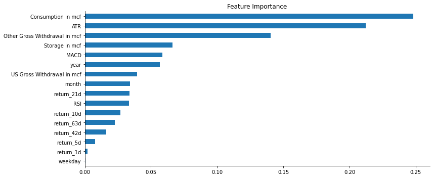
Using the builtin features_importances_ attribute from our model we can see that the most impactful params are:
- ATR
- NG consumption
- Other States Gross Withdrawal
- US Gross Withdrawal
- year
- MACD
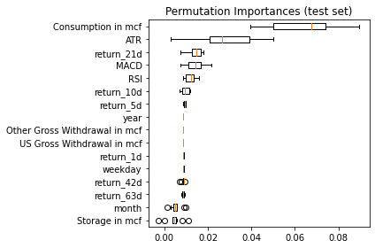
To have a more holistic view of the importance of the features, we can use two others functions provided by
sklearn: permutation_importance and partial_dependence.
from sklearn.inspection import permutation_importance, partial_dependence

result = permutation_importance(model, X_test, y_test.target_21d, n_repeats=10, n_jobs=-1, max_samples=0.3)

sorted_idx = result.importances_mean.argsort()

fig, ax = plt.subplots()
ax.boxplot(result.importances[sorted_idx].T,
           vert=False, labels=X.columns[sorted_idx])
ax.set_title("Permutation Importances (test set)")
fig.tight_layout()
plt.show()
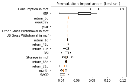
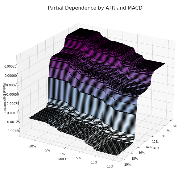
Partial dependence
Partial dependence plots (PDP) show the dependence between the target response and a set of input features of interest, marginalizing over the values of all other input features (the ‘complement’ features). Intuitively, we can interpret the partial dependence as the expected target response as a function of the input features of interest.
Partial dependence between the ATR and MACD
What is really significant in the image below is the gap in the partial dependence values when the approaches values between 0.16 and 0.14.
sns.set_style('whitegrid')
targets = ['ATR', 'MACD']
pdp, axes = partial_dependence(estimator=model,
                               features=targets,
                               X=X_test,
                               grid_resolution=100)

XX, YY = np.meshgrid(axes[0], axes[1])
Z = pdp[0].reshape(list(map(np.size, axes))).T

fig = plt.figure(figsize=(14, 8))
ax = Axes3D(fig)
surface = ax.plot_surface(XX, YY, Z,
                          rstride=1,
                          cstride=1,
                          cmap=plt.cm.BuPu,
                          edgecolor='k')
ax.set_xlabel('ATR')
ax.set_ylabel('MACD')
ax.set_zlabel('Partial Dependence')
ax.view_init(elev=22, azim=30)
ax.yaxis.set_major_formatter(FuncFormatter(lambda y, _: '{:.0%}'.format(y)))
ax.xaxis.set_major_formatter(FuncFormatter(lambda y, _: '{:.0%}'.format(y)))

# fig.colorbar(surface)
fig.suptitle('Partial Dependence by ATR and MACD', fontsize=16)
fig.tight_layout()
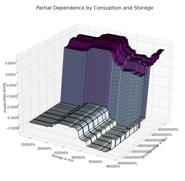
Partial dependence between the Consumption and Storage
sns.set_style('whitegrid')
targets = ['Consumption in mcf', 'Storage in mcf']
pdp, axes = partial_dependence(estimator=model,
                               features=targets,
                               X=X_test,
                               grid_resolution=100)

XX, YY = np.meshgrid(axes[0], axes[1])
Z = pdp[0].reshape(list(map(np.size, axes))).T

fig = plt.figure(figsize=(14, 8))
ax = Axes3D(fig)
surface = ax.plot_surface(XX, YY, Z,
                          rstride=1,
                          cstride=1,
                          cmap=plt.cm.BuPu,
                          edgecolor='k')
ax.set_xlabel('Consumption in mcf')
ax.set_ylabel('Storage in mcf')
ax.set_zlabel('Partial Dependence')
ax.view_init(elev=22, azim=30)
ax.yaxis.set_major_formatter(FuncFormatter(lambda y, _: '{:.0%}'.format(y)))
ax.xaxis.set_major_formatter(FuncFormatter(lambda y, _: '{:.0%}'.format(y)))

# fig.colorbar(surface)
fig.suptitle('Partial Dependence by Consuption and Storage', fontsize=16)
fig.tight_layout()
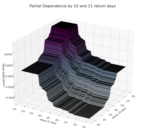
Partial Dependence between 10 and 21 return days
sns.set_style('whitegrid')
targets = ['return_10d', 'return_21d']
pdp, axes = partial_dependence(estimator=model,
                               features=targets,
                               X=X_test,
                               grid_resolution=100)

XX, YY = np.meshgrid(axes[0], axes[1])
Z = pdp[0].reshape(list(map(np.size, axes))).T

fig = plt.figure(figsize=(14, 8))
ax = Axes3D(fig)
ax.plot_surface(XX, YY, Z,
                    rstride=1,
                    cstride=1,
                    cmap=plt.cm.BuPu,
                    edgecolor='k')
ax.set_xlabel('return 10 days')
ax.set_ylabel('return 21 days')
ax.set_zlabel('Partial Dependence')
ax.view_init(elev=22, azim=30)
ax.yaxis.set_major_formatter(FuncFormatter(lambda y, _: '{:.0%}'.format(y)))
ax.xaxis.set_major_formatter(FuncFormatter(lambda y, _: '{:.0%}'.format(y)))

fig.suptitle('Partial Dependence by 10 and 21 return days', fontsize=16)
fig.tight_layout()
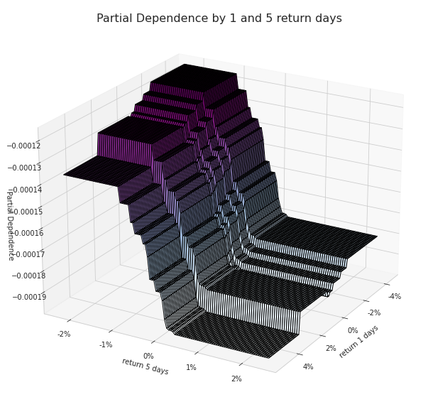
Partial Dependence between 1 and 5 return days
sns.set_style('whitegrid')
targets = ['return_1d', 'return_5d']
pdp, axes = partial_dependence(estimator=model,
                               features=targets,
                               X=X_test,
                               grid_resolution=100)

XX, YY = np.meshgrid(axes[0], axes[1])
Z = pdp[0].reshape(list(map(np.size, axes))).T

fig = plt.figure(figsize=(14, 8))
ax = Axes3D(fig)
ax.plot_surface(XX, YY, Z,
                    rstride=1,
                    cstride=1,
                    cmap=plt.cm.BuPu,
                    edgecolor='k')
ax.set_xlabel('return 1 days')
ax.set_ylabel('return 5 days')
ax.set_zlabel('Partial Dependence')
ax.view_init(elev=22, azim=30)
ax.yaxis.set_major_formatter(FuncFormatter(lambda y, _: '{:.0%}'.format(y)))
ax.xaxis.set_major_formatter(FuncFormatter(lambda y, _: '{:.0%}'.format(y)))

fig.suptitle('Partial Dependence by 1 and 5 return days', fontsize=16)
fig.tight_layout()
Partial Dependence between NG Consuption and ATR
sns.set_style('whitegrid')
targets = ['Consumption in mcf', 'ATR']
pdp, axes = partial_dependence(estimator=model,
                               features=targets,
                               X=X_test,
                               grid_resolution=100)

XX, YY = np.meshgrid(axes[0], axes[1])
Z = pdp[0].reshape(list(map(np.size, axes))).T

fig = plt.figure(figsize=(14, 8))
ax = Axes3D(fig)
ax.plot_surface(XX, YY, Z,
                          rstride=1,
                          cstride=1,
                          cmap=plt.cm.BuPu,
                          edgecolor='k')
ax.set_xlabel('Consumption in mcf')
ax.set_ylabel('ATR')
ax.set_zlabel('Partial Dependence')
ax.view_init(elev=22, azim=30)
ax.yaxis.set_major_formatter(FuncFormatter(lambda y, _: '{:.0%}'.format(y)))
ax.xaxis.set_major_formatter(FuncFormatter(lambda y, _: '{:.0%}'.format(y)))

fig.suptitle('Partial Dependence by Consuption and ATR', fontsize=16)
fig.tight_layout()

Comparing the two most important features identified before (the ATR and the Consumption) we can clearly we can see not only higher partial dependence values but also a well-defined pattern. As the ATR and the Consuption are approaching lower values the partial dependence grows, the opposite happens when the opposite conditions occur.
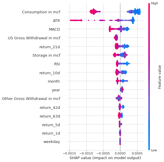
Shap Values
Shapley values originated in game theory as a technique for assigning a value to each player in a collaborative game that reflects their contribution to the team’s success. SHAP values are an adaptation of the game theory concept to tree-based models and are calculated for each feature and each sample. They measure how a feature contributes to the model output for a given observation. For this reason, SHAP values provide differentiated insights into how the impact of a feature varies across samples, which is important given the role of interaction effects in these nonlinear models.
Shapley values are computed by introducing each feature, one at a time, into a conditional expectation function of the model’s output, \(f_x(S) = \mathbb{E}[f(X) | do(X_s = x_s)]\), and attributing the change produced at each step to the feature that was introduced; then averaging this process over all possible feature orderings.
import shap

explainer = shap.TreeExplainer(model)
shap_values = explainer.shap_values(X=X_test)

shap.summary_plot(shap_values, X_test, show=False)
plt.tight_layout()
shap.summary_plot(shap_values, X_test, plot_type="bar",show=False)
plt.tight_layout()
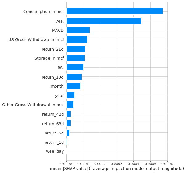
The Shap values that we are seeing in the two images are confirming the most important features that we’ve identified before, which are: ATR, Consumption, Other Gross Withdrawal, US Gross Withdrawal, year and the MACD.
What Shap values are telling us more is how each feature is positively/negatively impact the output. We can see from the first picture that:
- lower values of ATR usually lead to better returns, while when the ATR is higher the opposite tend to happend
- we can say the same thing about the Consumption
- earlier months often yield to worse result
- lower values of MACD are positively correlated to higher model output values, like the atr
- US Gross Withdrawal Values that have highly deviated from the mean tend to yield to positive returns, while closer values to mean often yield negative returns
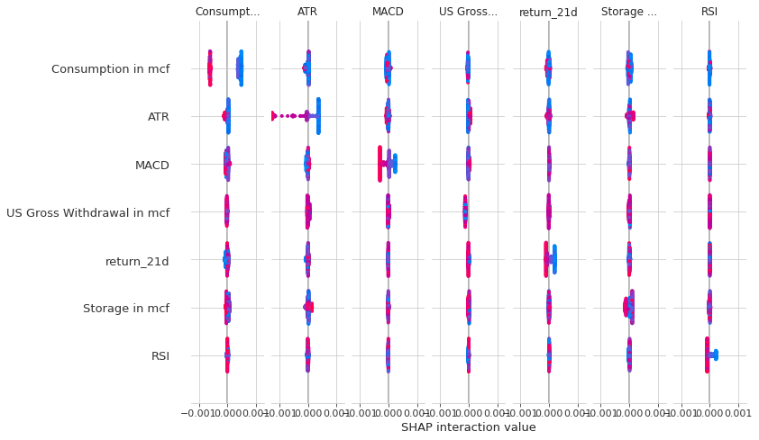
shap_interaction_values = explainer.shap_interaction_values(X_test)

shap.summary_plot(shap_interaction_values, X_test)
Backtesting
Now that we trained and evaluated the most important features of our model let’s use it in a trading strategy on the natural gas futures.
The strategy that I’m going to implement is the following:
Since the model has been trained to predict the return of the next n days I’m going to use a window of predictions (for instance a 10-day window) and I’m going to look for a peak positive or negative in that window of predictions. Once I’ve identified the peak, if the peak is positive I’m going to submit a buy order, while if the peak is negative I’m going to submit a sell order.
So, what I’m doing is to leverage the forecast of the model for the next period to submit an order.
The money management and risk management rule that the startegy is going to use are the following:
- Money management: 5% of the total equity per trade
- Risk management: a trailing stop that is looking at the low of the third previous day and subtact the current atr multiplied by 1.5
Let’s see how it works in practice.
Little Discaimer: the backtesting engine that I’ve used treat futures like a stock so don’t expect the results to be real, because it doesn’t take into account all the varibles that you should look for when trading futures. This strategy is only for didactical purpouse.
backtest_data = data.loc['2019':'2021']
import math

from scipy.signal import find_peaks

from backtesting import Backtest, Strategy

import tulipy as tu
def return_indicator(values, data_len: int):
    a = np.empty((data_len - len(values),))
    a[:] = np.nan
    return np.concatenate([a, values])

def get_atr(data: pd.DataFrame, n: int):
    atr = tu.atr(data.High, data.Low, data.Close, n)
    return return_indicator(atr, len(data))
class RFModelStrategy(Strategy):
    risk = 5 # 5% of the total amount per trade
    pred_len = 18
    atr_stop_multiplier = 1.5
    trailingATRLen = 5


    def init(self):
        super(RFModelStrategy, self).init()
        self.lookback = 3
        self.pointvalue = 10

        self.model = model
        self.atr = self.I(get_atr, self.data, 14, plot=False)
        self.trailingAtr = self.I(get_atr, self.data, self.trailingATRLen, plot=False)
        self.forecasts = self.I(lambda: np.repeat(np.nan, len(self.data)), name='forecast', color='red')

    def get_signal(self, predictions):
        if np.sum(predictions < 0, axis=0) / self.pred_len > 0.75:
            neg_peaks, _ = find_peaks(-predictions, width=2)

            if len(neg_peaks) != 0:
                return 'Sell'

        elif np.sum(predictions > 0, axis=0) / self.pred_len > 0.75:
            peaks, _ = find_peaks(predictions, width=2)

            if len(peaks) != 0:
                return 'Buy'

        return 'No signal'

    def next(self):
        X, _ = get_X_y(self.data.df)
        predictions = self.model.predict(X[-self.pred_len:])

        self.forecasts[-1] = self.model.predict(X[-2:])[0]

        if len(self.trades) == 0:
            signal = self.get_signal(predictions)

            if signal == 'Sell':
                self.sell(size=self.get_position_size())
            elif signal == 'Buy':
                self.buy(size=self.get_position_size())
        else:

            signal = self.get_signal(predictions)

            if self.trades[0].is_long:
                if signal == 'Sell' or \
                        self.data.Low[-1] <= self.get_trailing_stop(long=True):
                    self.position.close()
                    if signal == 'Sell':
                        self.sell(size=self.get_position_size())
            else:
                if signal == 'Buy' or \
                        self.data.High[-1] >= self.get_trailing_stop(long=False):
                    self.position.close()
                    if signal == 'Buy':
                        self.buy(size=self.get_position_size())

    def get_position_size(self):
        return math.floor((self.risk / 100 * self.equity) / (self.atr * self.pointvalue))

    def get_trailing_stop(self, long: bool):
        if long:
            return np.max(self.data.Low[-self.lookback:]) - self.trailingAtr[-1] * self.atr_stop_multiplier
        else:
            return np.min(self.data.High[-self.lookback:]) + self.trailingAtr[-1] * self.atr_stop_multiplier
bt = Backtest(backtest_data, RFModelStrategy, cash=250_000, trade_on_close=True, commission=0.02)

stats = bt.run()

stats
Start                     2019-01-02 00:00:00
End                       2021-08-30 00:00:00
Duration                    971 days 00:00:00
Exposure Time [%]                    91.95231
Equity Final [$]                 288032.29994
Equity Peak [$]                  288032.29994
Return [%]                           15.21292
Buy & Hold Return [%]               45.537525
Return (Ann.) [%]                    5.462319
Volatility (Ann.) [%]                5.324367
Sharpe Ratio                         1.025909
Sortino Ratio                        1.634402
Calmar Ratio                         0.684179
Max. Drawdown [%]                   -7.983754
Avg. Drawdown [%]                   -0.844115
Max. Drawdown Duration      597 days 00:00:00
Avg. Drawdown Duration       31 days 00:00:00
# Trades                                   27
Win Rate [%]                        59.259259
Best Trade [%]                      42.785025
Worst Trade [%]                    -27.783283
Avg. Trade [%]                       2.143391
Max. Trade Duration          94 days 00:00:00
Avg. Trade Duration          33 days 00:00:00
Profit Factor                        1.743472
Expectancy [%]                       3.260092
SQN                                  1.563307
_strategy                     RFModelStrategy
_equity_curve                             ...
_trades                        Size  Entry...
dtype: object
bt.plot(filename='./tree_regressor_backtesting.html')


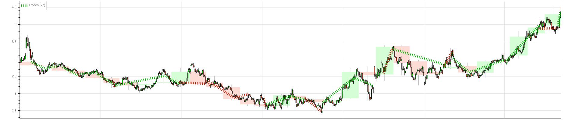


As we can see the strategy in the past two years is profitable, it has a decent rate of win rate (almost 60%), but it does not beat the buy and hold returns and the maximum drawdown duration is more than and year and a half(even though the maximum drawdown is 8%, which is pretty good).
References
- NHANES I Survival Model
- Long-Short Strategy, Part 4: How to interpret GBM results
- Preparing Alpha Factors and Features to predict Stock Returns
- Prediction stock returns with linear regression