Time series forecasting using CNNs

Usually, CNNs are linked to the whole field of computer vision, and that’s because in the past 10 years the best breakthrough in Computer vision is due to the use and improvement of the CNN architecture.

Today we are going to see how CNNs can be also applied to the problem of time series forecasting.

First and foremost we shall introduce what a time series is.

A time series is a sequential set of data points, measured typically over successive times. There are different categories regarding time series:

• univariate vs. multivariate: a time series containing records of a single variable is termed as univariate, but if records of more than one variable are considered then it is termed as multivariate.

• linear vs. non-linear: a time series model is said to be linear or non-linear depending on whether the current value of the series is a linear or non-linear function of past observation.

• discrete vs. continuous: in continuous time-series, observations are measured at every instance of time, whereas a discrete-time series contains observations measured at discrete points in time.

Here we are going to deal only with discrete time series.

The natural choice for sequence learning using Neural Net is to use an RNN. That’s because an RNN has a sequential structure so it seems more appropriate to model sequences. But on the flip side, because of their sequential structure, the training of an RNN cannot leverage the modern hardware used to train Neural Networks.

Another approach for tackling the sequence learning problem using Neural Network architectures is to use a variant of a CNN: a Temporal Convolutional Neural Network (TCN).

The distinguishing characteristic of TCNs are:

• The convolutions in the architecture are casual, meaning that there is no information “leakage” from future to past;
• The architecture can take a sequence of any length and map it to an output sequence of the same length, just as with an RNN.

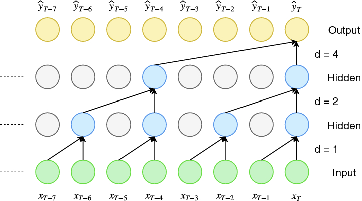
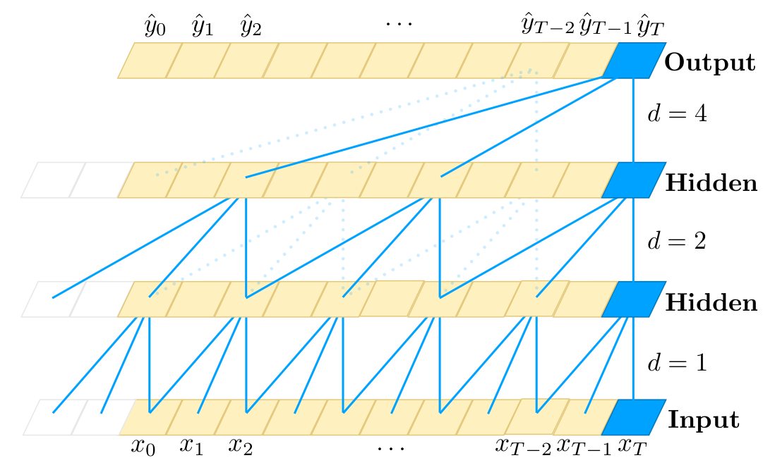
To achieve the first point, the TCN uses casual convolutions, convolutions where output at time $t$ is convolved only with elements from time $t$ and earlier in the previous layer. To accomplish the second point, the TCN uses a 1D fully-convolutional network architecture, where each hidden layer is the same length as the input layer, and zero padding of length (kernel size -1) is added to keep subsequent layers the same length as previous ones.

In other words TCN = 1D FCN + causal convolutions

an example of dilated convolution

A simple causal convolution is only able to look back in history with size linear in the depth of the network. This makes it challenging to apply the aforementioned causal convolution on sequence tasks, especially those requiring longer history. One possible solution here is to employ dilated convolutions that enable exponentially large receptive fields. More formally, for a 1-D sequence input $\mathbf{X} \in \mathbb{R}^n$ and a filter $f: \lbrace 0, \cdots, k -1 \rbrace \rightarrow \mathbb{R}$, the dilated convolution operation $F$ on element $s$ of the sequence is defined as:

where $d$ is the dilation factor, $k$ is the filter size, and $s - d \cdot i$ accounts for the direction of the past. Dilation is thus equivalent to introducing a fixed step between every two adjacent filter taps.

To ensure that some filter hits each input within the effective history, while also allowing for an extremely large history using deep networks $d$ is increased exponentially with the depth of the network.

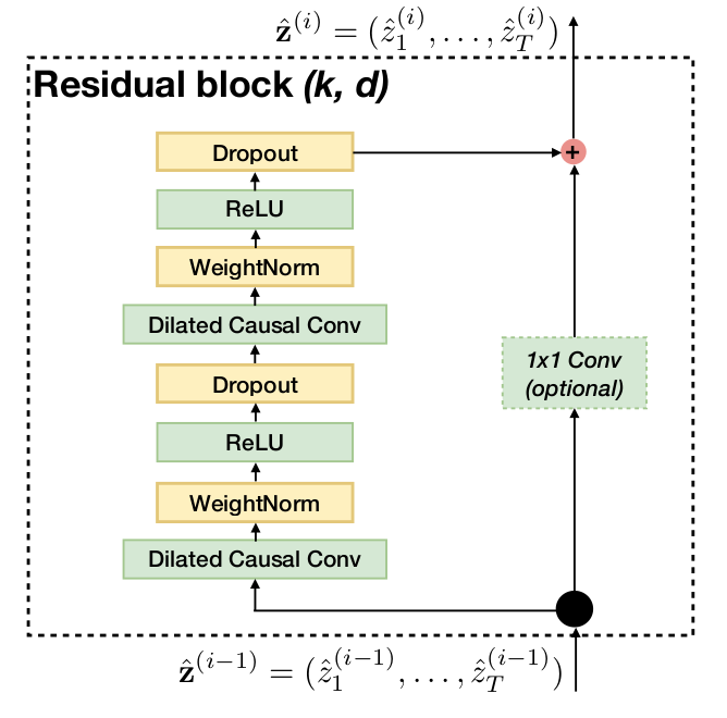
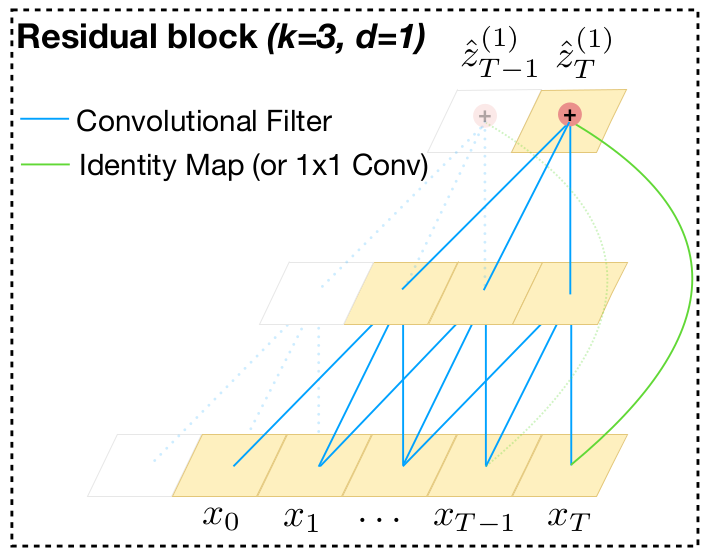
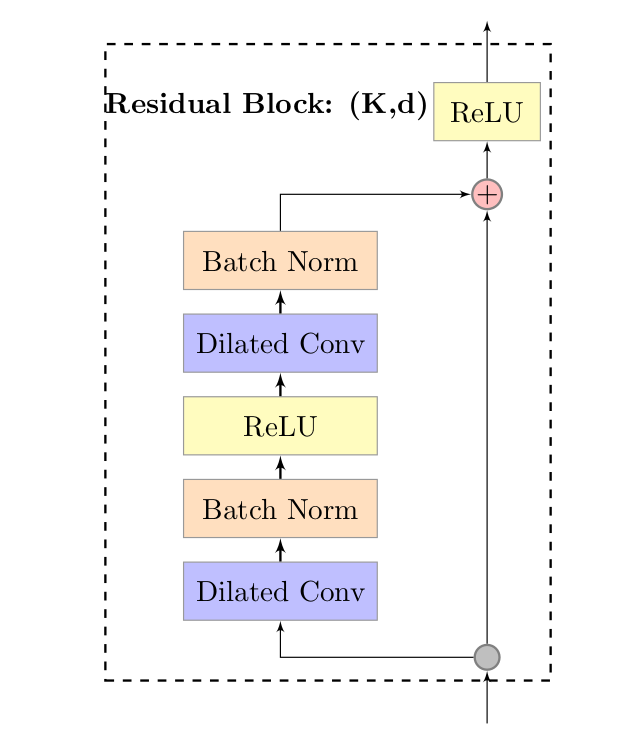
Another building block of the TCN architecture is the residual block. A residual block contains a branch leading out to a series of transformations $\mathcal{F}$, whose outputs are added to the input $\mathbf{x}$ of the block:

This effectively allows layers to learn modification to the identity mapping rather than the entire transformation, which has repeatedly been shown to benefit very deep networks.

To account for discrepant input-output widths, an additional 1x1 convolution is used to ensure that element-wise addition $\otimes$ receives tensors of the same shape.

The image below shows visually how a residual block is structured:

Let’s now see how well a TCN works in practice. I’m going to use as a target series the future continuous contract of natural gas.

Here I’m going to use darts which is a Python library for easy manipulation and forecasting of time series. It also provides a variety of models (including deep learning models) and it makes it easy to backtest models.

Let’s first import the libraries:

import numpy as np
import matplotlib.pyplot as plt
import pandas as pd

from darts import TimeSeries
from darts.utils.missing_values import fill_missing_values

filepath = '/content/drive/MyDrive/Datasets/trading/NG/HistoricalData_NG.csv'

ts_close = fill_missing_values(
    TimeSeries.from_csv(filepath, time_col='Date', value_cols='Close', freq='D'), 'auto')
ts_open = fill_missing_values(
    TimeSeries.from_csv(filepath, time_col='Date', value_cols='Open', freq='D'), 'auto')
ts_high = fill_missing_values(
    TimeSeries.from_csv(filepath, time_col='Date', value_cols='High', freq='D'), 'auto')
ts_low = fill_missing_values(
    TimeSeries.from_csv(filepath, time_col='Date', value_cols='Low', freq='D'), 'auto')
ts_volume = fill_missing_values(
    TimeSeries.from_csv(filepath, time_col='Date', value_cols='Volume', freq='D'), 'auto')

ts_close.plot()

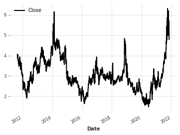
To make the training phase more stable is often useful to scaling the data that the network is going to receive as input. We are also going to use series of the Highest, Lowest and open daily prices. Those series could be useful as covariates series for the model.

from darts.dataprocessing.transformers import Scaler 
from darts.utils.timeseries_generation import datetime_attribute_timeseries

scaler = Scaler()
ts_transformed_close = scaler.fit_transform(ts_close)
ts_transformed_low = scaler.fit_transform(ts_low)
ts_transformed_open = scaler.fit_transform(ts_open)
ts_transformed_high = scaler.fit_transform(ts_high)

train, val = ts_transformed_close.split_after(pd.Timestamp('20200101'))
train_l, val_l = ts_transformed_low.split_after(pd.Timestamp('20200101'))
train_o, val_o = ts_transformed_open.split_after(pd.Timestamp('20200101'))
train_h, val_h = ts_transformed_high.split_after(pd.Timestamp('20200101'))

Now that the data is ready, let’s build the model:

from darts.models import TCNModel

tcn = TCNModel(
    n_epochs=125, 
    input_chunk_length=63,
    output_chunk_length=5, 
    dropout=0.1, 
    dilation_base=2, 
    weight_norm=True,
    kernel_size=3,
    num_filters=6,
    nr_epochs_val_period=1,
    random_state=0,
)

tcn.fit(
    series=train,
    past_covariates=train_l
)

As a past covariate series, I’ve decided to use the series of the lows, because it is always useful that the model is always aware of how worst the price could go. In finance you always have to prioritize to manage the risks and not the highest rewards possible, it is known that high rewards go hand in hand with higher risks.

Now that we’ve trained our model, let’s see how well it has done in the past.

pred_series = tcn.historical_forecasts(
    series=ts_transformed_close,
    start=pd.Timestamp('20200101'), 
    past_covariates=ts_transformed_low,
    forecast_horizon=1,
    stride=1,
    retrain=False,
    verbose=True,
    num_samples=1
)

100%|██████████| 682/682 [00:09<00:00, 69.51it/s]

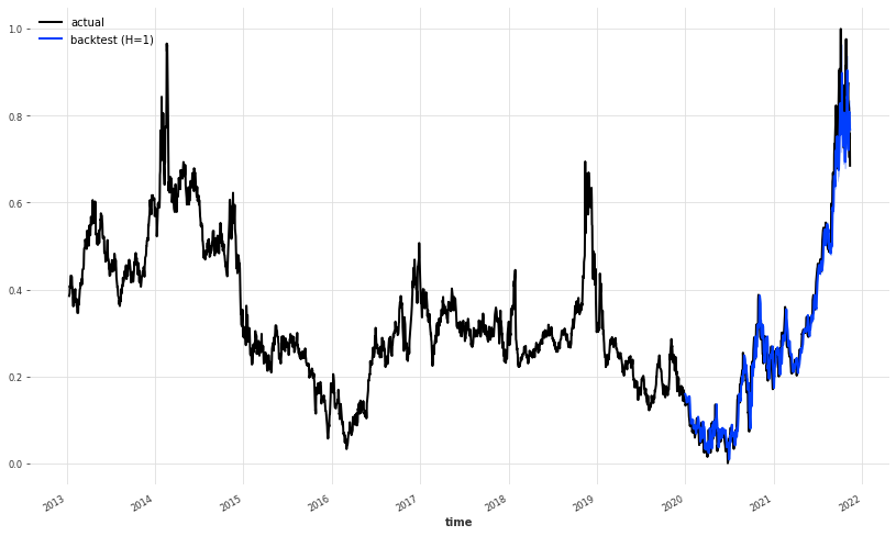
plt.figure(figsize=(14,8))

ts_transformed_close[500:].plot(label='actual')
pred_series.plot(label='backtest (H=1)', 
                 low_quantile=0.01,
                high_quantile=0.99)
plt.legend();

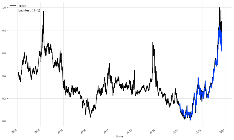
It seems like that the model, apart from the last part has done a pretty great job at predicting the future price of natural gas. Let’s take a look a the last part:

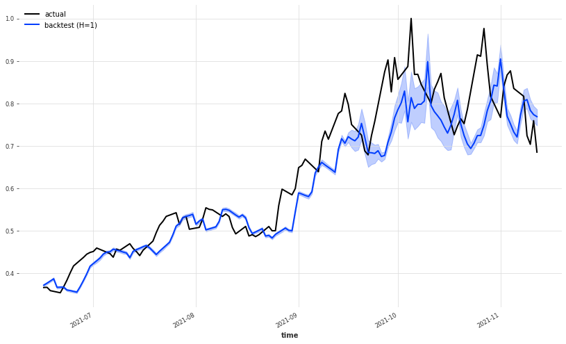
plt.figure(figsize=(14,8))

ts_transformed_close[-150:].plot(label='actual')
pred_series[-150:].plot(label='backtest (H=1)', 
                 low_quantile=0.01,
                high_quantile=0.99)
plt.legend();

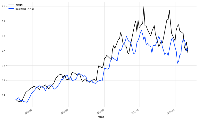
Despite being a little bit late from the real series, the model has done a great job at predicting the overall movements of the price, which is pretty insane if you think about it.

Probabilistic Forecasting with TCNs

TCNs are great but they don’t give an estimate about the uncertainty of their predictions, which can be very useful in some cases. Sometimes a range of values can be more meaningful than just a number.

The paper (Chen et al.) introduced a probabilistic forecasting framework based on convolutional neural network (CNN) for multiple related time series forecasting. This framework can be applied to estimate probability density under both parametric and non-parametric settings.

Giving a set of time series $\boldsymbol y_{1:t} = \lbrace y_{1:t}^{(i)}\rbrace_{i=1}^{N}$, we denote the future time series as $\boldsymbol y_{(t+1):(t+\Omega)} = \lbrace y_{(t+1):(t+\Omega)}^{(i)}\rbrace_{i=1}^{N}$, where $N$ is the number of series, $t$ is the length of the historical observations and $\Omega$ is the length of the forecasting horizon. The goal of the model is to predict the distribution of the future time series by directly forecast the joint distibution:

While time series data usually have systematic patterns such as trend and seasonality, it is also crucial that a forecasting framework allows covariates $X_{t+\omega}^{(i)}$ (where $\omega = 1, \cdots, \Omega$ and $i = 1, \cdots, N$) that include additional information to the direct forecasting strategy in \eqref{joint-pro-eq}. The joint distribution of the future incorporating the covariates becomes:

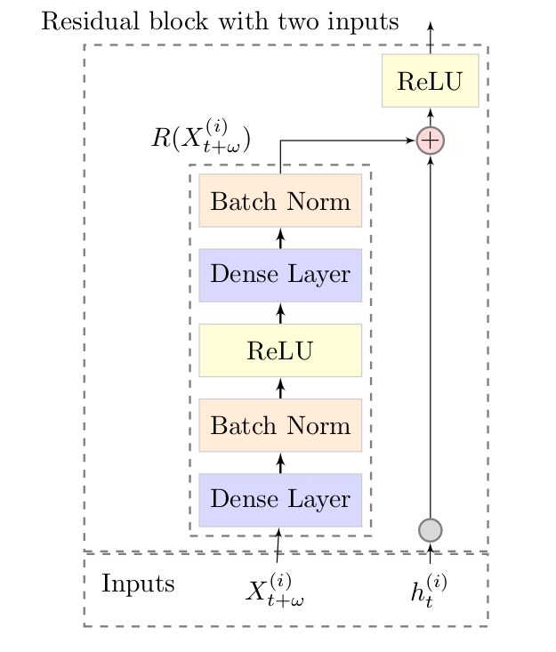
The neural network architecture is an encoder-decoder architecture, where the encoder consists of a vanilla TCN and the decoder includes two parts. The first part is the variant of a residual neural network, the module resnet-v. The second part is a dense layer that maps the output of the resnet-v to the probabilistic forecast. Figure \ref{fig:deep-tcn-arch} visually shows the architecture of a deep TCN.

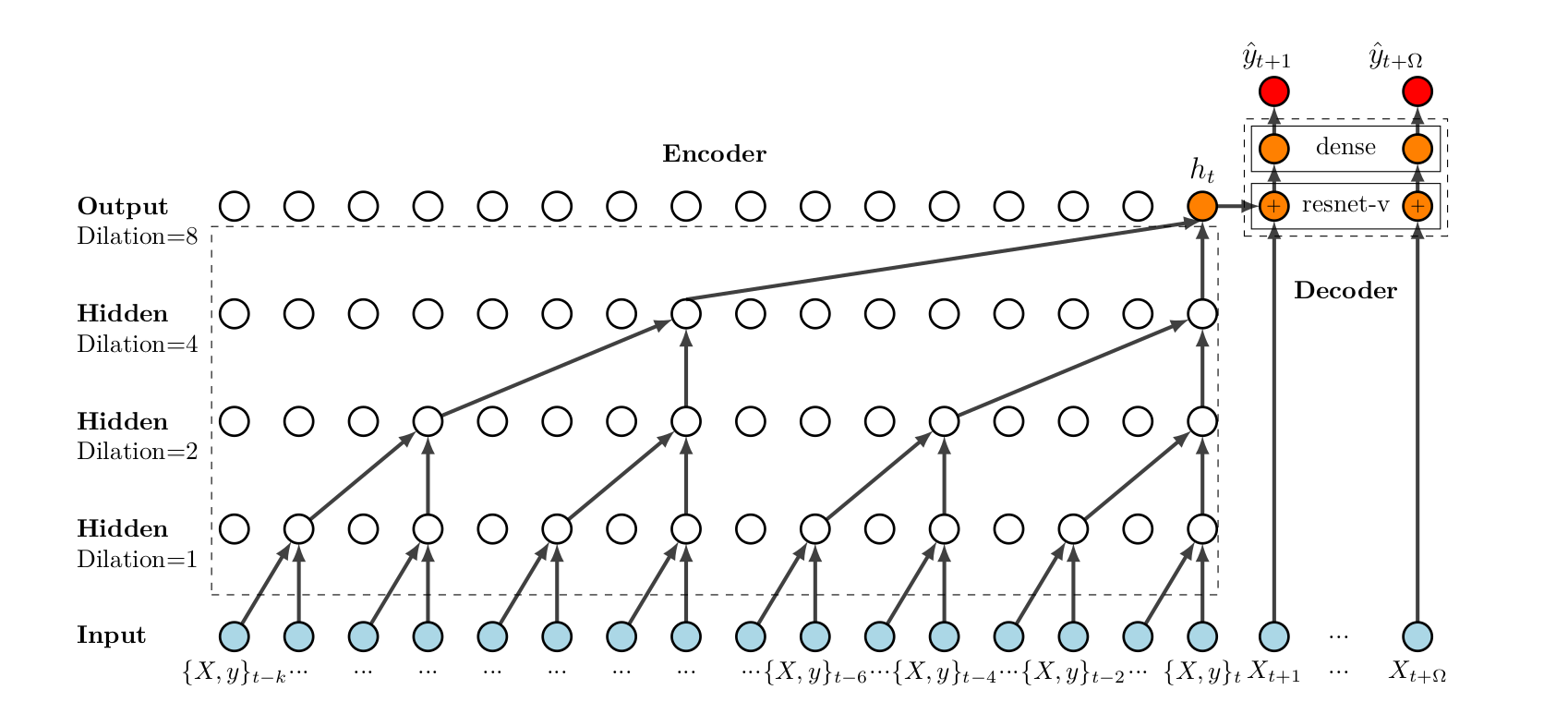Architecture of DeepTCN. Encoder part: stacked dilated causal convolutional nets are constructed to capture the long-term temporal dependencies. Decoder part: the decoder includes a variant of the residual block (referred to as resnet-v, shown as $\otimes$) and an output dense layer. The module resnet-v is designed to integrate the output of a stochastic process of historical observations and future covariates. Then the output dense layer is adopted to map the output of resnet-v into our final forecasts.

• Encoder module. Residual blocks are taken as the ingredient. Each residual block consists of two layers of dilated causal convolutions, the first of which is followed by a batch normalization and ReLU and the second of which is follow by another batch normalization. The output is taken as the input of the residual block, followed by another ReLU.

• Decoder module. $h_t^{(i)}$ output of the encoder, $X_{t+\omega}^{(i)}$ are the future covariates, and $R(\cdot)$ is the nonlinear function applied on is the $X_{t+\omega}^{(i)}$. For the residual function $R(\cdot)$, we first apply a dense layer and a batch normalization to project the future covariates. Then a ReLU activation is applied followed by another dense layer and batch normalization.

Probabilistic Forecasting Framework

Neural networks enjoy the flexibility to produce multiple outputs. In the DeepTCN framework, for each future observation, the output dense layer in the decoder can produce $m$ outputs: $Z=(z^1, \cdots, z^m)$, which represent the parameter set of the hypothetical distribution of interest. There are two possible probabilistic frameworks that can be used: the parametric framework and the non-parametric framework. In the parametric framework probabilistic forecast of future observations can be achieved directly by predicting the parameters of the hypothetical distribution based on maximum likelihood estimation. The non-parametric approach produces a set of forecasts corresponding to quantile points of interest with $Z$ representing the quantile forecast

Non-parametric approach

In the non-parametric framework, the forecast can be obtained by quantile regression. Models are trained to minimize the quantile loss, which is defined as

where $(y)^+ = \max(0, y)$ and $q \in (0,1)$. Given a set of quantile levels $Q= (q_1, \cdots, q_m)$, the $m$ corresponding forecast can be obtained by minimizing the total quantile loss defined as

Parametric approach

For the parametric approach, given the predetermined distribution, the maximum likelihood estimation is applied to estimate the corresponding parameters. Take Gaussian distribution for example, for each target value $y$, the network outputs the parameters of the distribution, namely the mean $\mu$ and the standard deviation $\sigma$. The negative log-likelihood function is then constructed as the loss function:

Let’s now see how the Probabilistic TCN perform on the same time series forecasting problem that we’ve seen above:

from darts.utils.likelihood_models import GaussianLikelihood

deep_tcn = TCNModel(
    n_epochs=125, 
    input_chunk_length=63,
    output_chunk_length=5, 
    dropout=0.1, 
    dilation_base=2, 
    weight_norm=True,
    kernel_size=3,
    num_filters=6,
    nr_epochs_val_period=1,
    random_state=0,
    likelihood=GaussianLikelihood()
)

deep_tcn.fit(
    series=train,
    past_covariates=train_l,
)

pred_series = deep_tcn.historical_forecasts(
    series=ts_transformed_close,
    start=pd.Timestamp('20200101'), 
    past_covariates=ts_transformed_low,
    forecast_horizon=1,
    stride=1,
    retrain=False,
    verbose=True,
    num_samples=200
)

100%|██████████| 682/682 [00:27<00:00, 25.19it/s]

plt.figure(figsize=(14,8))

ts_transformed_close[500:].plot(label='actual')
pred_series.plot(label='backtest (H=1)', 
                 low_quantile=0.01,
                high_quantile=0.99)
plt.legend();

plt.figure(figsize=(14,8))

ts_transformed_close[-150:].plot(label='actual')
pred_series[-150:].plot(label='backtest (H=1)', 
                 low_quantile=0.01,
                high_quantile=0.99)
plt.legend();

While the main prediction has seemed to improve from the non-probabilist version, the fact that it immediately catches the eye is that we have a sort of confidence interval about the prediction which is super useful. In this way, we don’t only have just a mere prediction of what could be the future price but we have an interval of uncertainty about that prediction. Notice that the uncertainty interval opens up when the volatility is increasing, maybe here using the lows series is even more useful than before (lower prices in a trading day often means that higher volatility has occurred during the day).