Basics of Reinforcement Learning: MDPs

After introducing Reinforcement learning, a question that may arise is: How are we going to represent those Reinforcement learning problems?

Well, mathematics provides us with all the tools that we need, and, for this purpose, it gives us a framework for modeling decision-making in situations where the outcomes are partially random and part under the control of a decision-maker. This framework is called the Markov Decision Process (MDP) and is an extension of the Markov Chain ideated by the Russian mathematician Andrey Markov.

But before introducing the MDP, let’s first talk about his foundation the Markov Chain. A Markov Chain is a stochastic model describing a sequence of possible events in which the probability of each event depends only on the state attained in the previous event. Formally speaking is defined as a tuple \( \langle S, P \rangle \) where:

\( S \) is a finite set of state of the process,
\( P \) is the transition probability matrix For a Markov stats \( s \) and successor state \( s’ \), the state transition matrix is defined by a formula.

\[P_{ss'} = \mathbb{P}[S_{t+1} = s' | S_t = s]\]

The State transition matrix \( P \) defines transition probabilities from state \( s \) to all successor state \( s’ \).

\[P = \begin{bmatrix} P_{11} & \cdots & P_{1n} \\ \vdots & & \vdots \\ P_{n1} & \cdots & P_{nn} \end{bmatrix}\]

Another important thing is that an Markov Chain must satisfy the Markov property. This property can be summarized as follows: “The future is independent of the past of the given present”.

Mathematically speaking, a stochastic process has the Markov property if the conditional probability distribution of future states of the process depends only upon the present state, not on the sequence of events that preceded it.

A state is Markov if and only if:

\[\mathbb{P}[S_{t+1} | S_t] = \mathbb{P}[S_{t+1} | S_1, \cdots, S_t ]\]

But why the Markov property is even useful in the first place?

Well, if you think about it a Markov state summarizes the past sensation compactly, yet in such a way that all relevant information is retained. This is sometimes also referred to as an “independence of path” property because all that matters is in the current state signal; its meaning is independent of the history of signals that have led up to it. So the importance of the Markov property in reinforcement learning is that the decisions and values are assumed to be a function only of the current state.

But now that we have understand what is a Markov chain let’s see an example of a Markov chain.

markov-aids

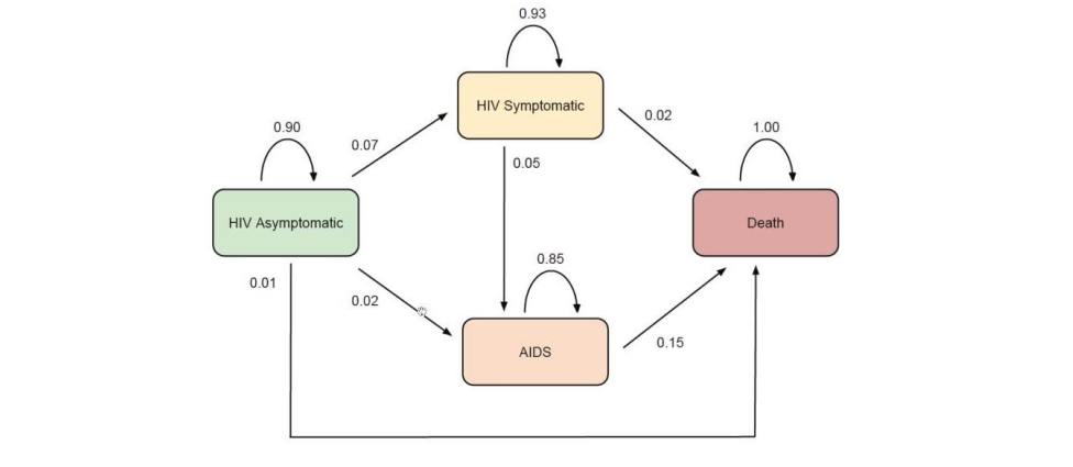
The matrix above gives the probabilities of moving from 1 health state to another in 1 year. The transition probability matrix of the above Markov chain is:

p_matrix = [
    [0.90, 0.07, 0.02, 0.01],
    [0, 0.93, 0.05, 0.02],
    [0, 0, 0.85, 0.15],
    [0, 0, 0, 1.00]
    ]

Let’s now assume that the current helth states for a group are:

85% asymptomatic
10% symptomatic
5% AIDS
0% death

What will be the % in each health state in 1 year? Well if you think about it, we can summarize the group’s health state in a vector and just multiply the vector for the transition probabilities matrix. Let’s do this using numpy!

import numpy as np 

v = np.array([0.85, 0.10, 0.05, 0])
p_matrix = np.array([
    [0.90, 0.07, 0.02, 0.01],
    [0, 0.93, 0.05, 0.02],
    [0, 0, 0.85, 0.15],
    [0, 0, 0, 1.00]
    ])

print(v @ p_matrix)

array([0.765 , 0.1525, 0.0645, 0.018 ])

Pretty easy right?

Now that we understand how the Markov chain work we can start to talk about the MDPs.

Markov Decision Process

Formally speaking, a Markov decision process is a 4-tuple \( \langle S, A, P_a, R_a \rangle \) dove:

\( S \) is a finite set of states called state space
\( A \) is a finite set of actions called action space
\( P_a(s , s’) \) is the state transition probability matrix, so is the probability that action \( a \) in state \( s \) at time \( t \) will lead to state \( s’ \) at time \( t + 1 \).
\( R_a(s, s’) \) is a reward function, hence the immediate reward received after transitioning from state \(s \) to state \( s’ \), due to action \( a \)

The objective of our agent in a MDP is to maximise the expected returns, hence the agent wants to maximise the sum of rewards over time. A first naive way of mathematically define the expected return \( G_t \) is, as I said before, simply putting them as the sum of the rewards:

\[G_t = R_{t + 1} + R_{t + 2} + R_{t + 3} + \cdots + R_T\]

where \( T \) is a final time step. The definition of return is nice, but in reinforcement learning a variant of it is used. This variant is called discounted return, and is defined as follows:

\[G_T = R_{t + 1} + \gamma R_{t + 2} + \gamma^2 R_{t + 3} + \cdots = \sum_{k = 0}^{\infty} \gamma^k R_{t + k + 1}\]

here’s the \( 0 \le \gamma \le 1 \) is called the discount rate. This parameter has a nice interpretation: it basically determines the present value of future rewards: a reward received k time steps in the future is worth only \(γ^{k−1} \) times what it would be worth if it were received immediately. If \( \gamma = 0 \), the agent is “myopic” in being concerned only with maximizing immediate rewards, while the more \( \gamma \) is closer to 1 the more the agent takes future rewards into account more strongly.

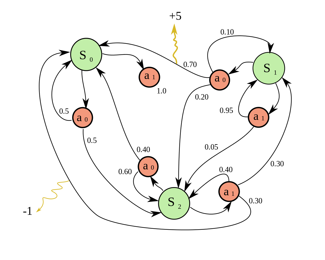
An Example of an MDP

Let’s assume that we can turn a recycling robot into a simple MDP. And let’s also assume hat the agent makes a decision at times determined by external events. At each such time the robot decides whether it should (1) actively search for a can, (2) remain stationary and wait for someone to bring it a can, or (3) go back to home base to recharge its battery. Suppose the environment works as follows. The best way to find cans is to actively search for them, but this runs down the robot’s battery, whereas waiting does not. Whenever the robot is searching, the possibility exists that its battery will become depleted. In this case the robot must shut down and wait to be rescued.

The agent makes its decisions solely as a function of the energy level of the battery. It can distinguish two levels, high and low, so that the state set is \( S = { \mbox{high}, \mbox{low} } \). Let us call the possible decisions—the agent’s actions— wait, search, and recharge. When the energy level is high, recharging would always be foolish, so we do not include it in the action set for this state. The agent’s action sets are

\[A(\mbox{high}) = \{ \mbox{search}, \mbox{wait} \} \\\] \[A(\mbox{low}) = \{ \mbox{search}, \mbox{wait}, \mbox{recharge} \}\]

Regarding the rewards that the robot will get from the enviroment of course the order must be the following

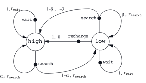
\[r_{search} > r_{wait}\]

becuase intuentivetly the robot will get more can if it seach in the enviroment instead of doing nothing. çet also be \( \alpha \) the probability that the energy level will stay after searching and \( 1 - \alpha \) the probabilty of reduces its battery level to low after searching. Similarly let be \( \beta \) the probability of staying low when searching with low level of battery and \( 1 - \beta \) the probability of depleting its battery after searching. Of course the action will give a negative rewards to the robot, because we want our robot to be smart, so it doesn’t have to be restore by a human.

That’s the resulting MDP:

robot-mdp

Policy

As you might know the policy in reinforcement learning fully defines the agent behaiour. “It tells at the agent what to do, what action to take in a specific state”. Defining it mathematically a policy \( \pi \) is a distribution over action given states,

\[\pi (a | s) = \mathbb{P}[A_t = a | S_t = s]\]

In the context of MDPs a policy dependes on the current state, and the by the history of the action and state of the agents, so in the MDPs policies are stationaries:

\[A_t \sim \pi( \cdot | S_t), \forall t > 0\]

Value Functions

Now that we know what is an MDP and we had define policy in the context of the MDPs, it may be useful to define some metrics that will help us to solve and describe these MDPs. Almost all reinforcement learning algorithms involve estimating value functions - functions of state that estimate how good it is for the agent to be in a given state. Here’s the notion of “how good” is defined in terms of future rewards that can be expected, or, to be precise, in terms of expected return. Given a policy \( \pi \), we define the value of a state s under \( \pi \) formally as :

\[v_{\pi} (s) = \mathbb{E}_{\pi}[G_t | S_t = s] = \mathbb{E}_{\pi}[ \sum_{k = 0}^{\infty} \gamma^k R_{t + k + 1} | S_t = s]\]

where here \( \mathbb{E} \) denotes the expected values of a random variable given that the agent follows policy \( \pi \), and \( t \) is any time step. We call the function \( v_\pi \) the state-value function for policy \( \pi \).

Action-Value Functions

Similarly, we define the value of taking action \( a \) in state \( s \) under a policy \( \pi \), denoted by \( q_{\pi}(s, a) \), as the expected return starting form \( s \), taking the action \( a \), and thereafter following policy \( \pi \):

\[q_{\pi} (s, a) = \mathbb{E}_{\pi}[G_t | S_t = s, A_t = a] = \mathbb{E}_{\pi}[ \sum_{k = 0}^{\infty} \gamma^k R_{t + k + 1} | S_t = s, A_t = a]\]

We call the function \( q_{\pi} \) the action-value function for policy \( \pi \).

The value functions \( v_\pi \) and \( q_\pi \) can be estimated from experience. For example, if an agent follows policy \( \pi \) and maintains an average, for each state encountered, of the actual returns that have followed that state, then the average will converge to the state’s value, \( v_\pi(s) \), as the number of times that state is encountered approaches infinity. If separate averages are kept for each action taken in a state, then these averages will similarly converge to the action values, \( q_\pi(s, a) \).

Bellman Equation

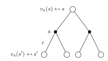
A fundamental property of value functions, and also of the action-value functions, used throughout reinforcement learning is that they satisfy particular recursive relationships. For any policy \( \pi \) and any state \( s \), the following consistency condition holds between the value of \( s \) and the value of its possible successor states:

\[\begin{aligned} v_\pi(s) &= \mathbb{E}[G_t \vert S_t = s] \\ &= \mathbb{E}_\pi [R_{t+1} + \gamma R_{t+2} + \gamma^2 R_{t+3} + \dots \vert S_t = s] \\ &= \mathbb{E}_\pi [R_{t+1} + \gamma (R_{t+2} + \gamma R_{t+3} + \dots) \vert S_t = s] \\ &= \mathbb{E}_\pi [R_{t+1} + \gamma G_{t+1} \vert S_t = s] \\ &= \mathbb{E}_\pi [R_{t+1} + \gamma V(S_{t+1}) \vert S_t = s] \\ &= \sum_a \pi(a|s) (R_a(s) + \gamma \sum_{s' \in S} P_{ss'}^a v_\pi (s')) \\ \end{aligned}\]

The previous equation is called Bellman Expectation Equation for \( v_\pi \), and it states that the value of the start state, following policy \( \pi \), must equal the discounted value of the expected next state, plus the reward exepected along the way. Think of looking ahead from one state to its possible successor states.

Similarly the Bellman Expectation Equation is define \( q_\pi \) as follow:

\[\begin{aligned} q_\pi (s, a) &= \mathbb{E}_\pi [R_{t+1} + \gamma V(S_{t+1}) \mid S_t = s, A_t = a] \\ &= \mathbb{E}_\pi [R_{t+1} + \gamma \mathbb{E}_{a\sim\pi} Q(S_{t+1}, a) \mid S_t = s, A_t = a] \\ &= R_a(s) + \gamma \sum_{s' \in S} P_{ss'}^a \sum_{a' \in A} \pi (a' | s') q_\pi (s', a') \end{aligned}\]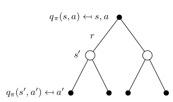

For example, let’s consider a simple grid world to illustrate the value function for out MDP. The cells of the grid correspond to the states of the environment. Actions that would take the agent off the grid leave its location unchanged, but also result in a reward of −1. Other actions result in a reward of 0, except those that move the agent out of the special states A and B. From state \( A \), all four actions yield a reward of +10 and take the agent to \( A’ \). From state \( B \), all actions yield a reward of +5 and take the agent to \( B’ \).

Suppose the agent selects all four actions with equal probability in all state. Using the Bellman Expectation equation, with \( \gamma = 0.9 \), for the value function we obtain the right grid shown below.

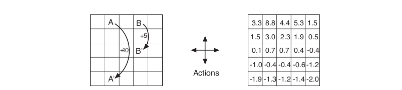
As you can notice near the lower edge we have negative values; this because there is an high probability of hitting the edge of the grid a get a reward of -1. While the highest value function is on the State \( B \), because the agent from \( B \) is taken to \( B’ \), which give us a reward of +5, and unlike \( A’ \) is not located on the edge of the grid, so it’s impossible that he’ll get negative rewards.

But since our task, and the reinforcement learning task in general, is to achieves a lot of reward over the long run, how we are going to find a policy that will get us to that goal?

We know that a policy \( \pi \) is defined to be better that or equal to a policy \( \pi’ \) if its expected return is greater that or equal to that \( \pi’ \) for all states. Hence, \( \pi \ge \pi’ \) if and only if \( v_\pi (s) \ge v_\pi’ (s), \forall s \in S \). There exists an policy \( \pi^* \) that is better that or equal to all other policies \( \pi^* \ge \pi \forall \pi\). This policy is called optimal policy.

All optimal policies achieve the optimal value function, defined as

\[v_{\pi^*}(s) = v_*(s) \hspace{25mm} \forall s \in S\]

Optimal policies also share the same optimal action-value function, defined as

\[q_{\pi^*}(s, a) = q_*(s, a) \hspace{25mm} \forall s \in S, \forall a \in A(s)\]

Because \( v^∗ \) is the value function for a policy, it must satisfy the self- consistency condition given by the Bellman equation for state values. Hence, similarly as before for the bellman expectation equation, the optimal value function are recursevly related:

\[\begin{aligned} v^*(s) &= \max_a q_* (s, a) \\ &= \max_a R_a(s) + \gamma \sum_{s' \in S} P_{ss'}^a v_* (s') \end{aligned}\]

Since we’re dealing with the optimal value function, this time the recusive equation is called Bellman Optimality Equation. The Bellman optimality equation for \( q_* \) is

\[\begin{aligned} q_* (s, a) &= R_a(s) + \gamma \sum_{s' \in S} P_{ss'}^a v_* (s') \\ &= R_a(s) + \gamma \sum_{s' \in S} P_{ss'}^a \max_a' q_* (s', a') \end{aligned}\]

For finite MDPs, the Bellman optimality equation of the value function has a unique solution independent of the policy. The Bellman optimality equation is actually a system of equations, one for each state, so if there are N states, then there are \( N \) equations in \( N \) unknowns.

Once one has \( v_∗ \) , it is relatively easy to determine an optimal policy. For each state \( s \), there will be one or more actions at which the maximum is obtained in the Bellman optimality equation. Any policy that assigns nonzero probability only to these actions is an optimal policy. If you have the optimal value function, \( v_* \), then the action that appear best after a one-step search will be optimal actions. So the optimal policy is acting greedly with respect to the optimal value function \( v_* \).

Having \(q_∗ \) makes choosing optimal actions still easier. With \(q_∗ \), the agent does not even have to do a one-step-ahead search: for any state \( s \), it can simply find any action that maximizes \(q_∗(s, a) \). So mathematically speaking using the optimal \( q_* \) values the policy is defined as:

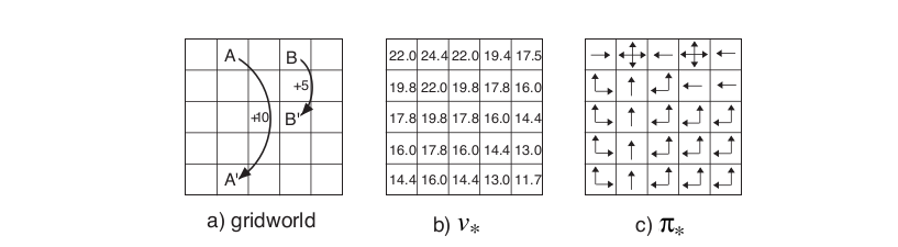
\[\pi_*(a | s) = \begin{cases} 1 & \quad \text{if } a = \text{arg}\max_{a \in A} q_*(s, a) \\ 0 & \quad \text{ otherwise} \end{cases}\]

Let’s consider again the grid world introduced before, and let’s suppose that we’ve solved the Bellman equation for \( v_* \). Solving the Bellman optimality equation provides one route to finding an optimal policy, and thus to solving the reinforcement learning problem. Here’s what the \( v_* \) and \( \pi_* \) are like:

References

Written on December 2nd , 2020 by Paolo

Feel free to share!